J.M.Pearce (talk | contribs) |
Sophivorus (talk | contribs) mNo edit summary |
||
| (31 intermediate revisions by 11 users not shown) | |||
| Line 1: | Line 1: | ||
[[File:va-spec.jpg|thumb]] | |||
{{MOST}} | {{MOST}} | ||
{{QAS notice}} | |||
= | |||
{{Project data | |||
| authors = O. Ormachea, A. Abrahamse, N. Tolavi, F. Romero, O. Urquidi, User:J.M.Pearce, Rob Andrews | |||
| instance-of = Photovoltaic system | |||
| location = Kingston, Canada; Cochabamba, Bolivia; Michigan, USA | |||
}} | |||
The goal for this '''Open Source Solar Spectrum Analyzer''' was to collaboratively design the mechanical and electronic controls for a direct/diffuse data acquisition of wavelength and tilt angle dependent solar flux. In this project we built and commissioned two systems (1 in Canada and 1 in Bolivia). The systems will adjust a fiber optic input from 0 to 90 degrees every ten degrees and measure global and diffuse by adjusting a shadow band in and out. These measurements occur every hour and have enough resolution to span the UV-VIS to NIR spectrum. | The goal for this '''Open Source Solar Spectrum Analyzer''' was to collaboratively design the mechanical and electronic controls for a direct/diffuse data acquisition of wavelength and tilt angle dependent solar flux. In this project we built and commissioned two systems (1 in Canada and 1 in Bolivia). The systems will adjust a fiber optic input from 0 to 90 degrees every ten degrees and measure global and diffuse by adjusting a shadow band in and out. These measurements occur every hour and have enough resolution to span the UV-VIS to NIR spectrum. | ||
In order to accomplish this, [[Queens Applied Sustainability Group]] in Kingston Ontario joined up with the La Universidad Privada Boliviana[http:// | In order to accomplish this, [[Queens Applied Sustainability Group]] in Kingston Ontario joined up with the La Universidad Privada Boliviana[http://upb.edu/] in Cochabamba, Bolivia. This partnership allowed for, in addition to the different location, an insight into how [[International collaboration protocol QAS|international collaboration]] can be implemented as well as ways to increase its productivity and efficiency. | ||
Our systems would be designed to be as similar as possible with an exception for their individual spectrometers. This will allow us to get comparable data from both sites in order to compare the geographic differences in the sun's radiation and the potential effects on solar photovoltaic output. | Our systems would be designed to be as similar as possible with an exception for their individual spectrometers. This will allow us to get comparable data from both sites in order to compare the geographic differences in the sun's radiation and the potential effects on solar photovoltaic output. | ||
This page describes how to build an automated spectrometer for recording solar spectra. It includes links to CAD files, design, software etc. It list all the components with links to purchase locations, includes calibration protocols, etc. Everything that is needed to replicate the two examples at UPB and in Canada....and a link to the data streams. | This page describes how to build an automated spectrometer for recording solar spectra. It includes links to CAD files, design, software etc. It list all the components with links to purchase locations, includes calibration protocols, etc. Everything that is needed to replicate the two examples at UPB and in Canada....and a link to the data streams. | ||
=Solar Spectrum Theory= | === Publication === | ||
O. Ormachea ; A. Abrahamse ; N. Tolavi ; F. Romero ; O. Urquidi ; J. M. Pearce ; R. Andrews; [http://proceedings.spiedigitallibrary.org/proceeding.aspx?articleid=1782233 Installation of a variable-angle spectrometer system for monitoring diffuse and global solar radiation]. ''Proc. SPIE 8785, 8th Iberoamerican Optics Meeting and 11th Latin American Meeting on Optics, Lasers, and Applications'', 87850M (November 18, 2013); DOI: http://dx.doi.org/10.1117/12.2025480 | |||
== Solar Spectrum Theory == | |||
The attenuation and transmission of light in the earth's atmosphere is important in many fields including: [[photovoltaic]] technology, agriculture, weather prediction and climate research. Due to the non-homogeneity of the earth's atmosphere and constantly changing solar geometry, the solar resource is variable and can have very different effects at geographically disparate sites on the planet. | The attenuation and transmission of light in the earth's atmosphere is important in many fields including: [[photovoltaic]] technology, agriculture, weather prediction and climate research. Due to the non-homogeneity of the earth's atmosphere and constantly changing solar geometry, the solar resource is variable and can have very different effects at geographically disparate sites on the planet. | ||
Solar irradiation is composed of a spectrum of light, which can broadly be divided into ultraviolet (UV), Visible (Vis), and Near Infrared (NIR) light. The light present at the edge of the earth's atmosphere, at what is called a 0 Air Mass (AM0) | Solar irradiation is composed of a spectrum of light, which can broadly be divided into ultraviolet (UV), Visible (Vis), and Near Infrared (NIR) light. The light present at the edge of the earth's atmosphere, at what is called a 0 Air Mass (AM0) is defined as the extraterrestrial insolation (Go), which is a consistently varying quantity, but generally defined as 1366.1 W/m<sup>2</sup> for engineering applications.<ref>C.A. Gueymard, The sun's total and spectral irradiance for solar energy applications and solar radiation models, Solar Energy. 76 (2004) 423-453.</ref> As the extraterrestrial spectrum travels through the earths atmosphere, it is attenuated by a variety of atmospheric constituents, including in descending order of their relative effects on solar transmission for a clear (cloudless) sky: Aerosols (ie scattering), Particulates (Rayleigh Scattering), Water Vapour, Ozone, Carbon Dioxide, and Oxygen. | ||
The level of the attenuation due to these atmospheric components is dependent on their relative concentrations and on the optical path length through which the solar irradiation passes. If the sun is directly overhead, the optical path length is said to be one air mass (AM1) as the solar elevation above the horizon decreases, the sun's irradiance must pass through a larger distance before reaching the surface, and therefore the air mass will increase. For many solar photovoltaic applications, the airmass of 1.5 (AM1.5) with an associated irradiance of 1000 W/m<sup>2</sup> (1 sun) is considered to be a standard atmospheric condition. A summary of the atmospheric constituents which can afford this condition and for a definition of the standard AM1.5 atmosphere (ASTM G-173), a comprehensive description can be found [http://rredc.nrel.gov/solar/spectra/am1.5/ here]. For an overview of the theory of solar resource measurements, see the related page on [[ | The level of the attenuation due to these atmospheric components is dependent on their relative concentrations and on the optical path length through which the solar irradiation passes. If the sun is directly overhead, the optical path length is said to be one air mass (AM1) as the solar elevation above the horizon decreases, the sun's irradiance must pass through a larger distance before reaching the surface, and therefore the air mass will increase. For many solar photovoltaic applications, the airmass of 1.5 (AM1.5) with an associated irradiance of 1000 W/m<sup>2</sup> (1 sun) is considered to be a standard atmospheric condition. A summary of the atmospheric constituents which can afford this condition and for a definition of the standard AM1.5 atmosphere (ASTM G-173), a comprehensive description can be found [http://rredc.nrel.gov/solar/spectra/am1.5/ here]. For an overview of the theory of solar resource measurements, see the related page on [[Solar resource measurement for PV applications]]. For a more in-depth overview of solar geometry, see the related page on [[The Solar Resource]] | ||
The spectral distribution of irradiance from the AM1.5 spectrum is shown below. <br> | The spectral distribution of irradiance from the AM1.5 spectrum is shown below.<br> | ||
[[ | [[File:Am1 5 spectrum.jpg|ASTM G173 AM1.5 spectrum]] | ||
== Solar attenuation == | |||
The attenuation of the solar resource in the atmosphere affects both the integrated (broadband) value of irradiation, as well as its distribution within the spectrum. Generally, an increase in Air Mass will tend to shift the spectrum towards "red" (Infrared), as can be observed due to the red sky at morning and evening. An increase in cloud cover will tend to shift the spectrum towards the "blue" (Ultraviolet), an effect which might be noticed when receiving a sunburn on a cloudy day. | |||
The attenuation of the solar resource in the atmosphere affects both the integrated (broadband) value of irradiation, as well as its distribution within the spectrum. Generally, an increase in Air Mass will tend to shift the spectrum towards "red" (Infrared), as can be observed due to the red sky at morning and evening. An increase in cloud cover will tend to shift the spectrum towards the "blue" (Ultraviolet), an effect which might be noticed when receiving a sunburn on a cloudy day. | |||
As can be seen in the above figure, the attenuation of irradiation also depends on the source of the irradiation. Direct & circumsolar refers to that irradiation which is not scattered in the atmosphere, and is specular in nature, meaning that it is directional and will form shadows when blocked. The Diffuse irradiation is irradiation which comes from the sky dome, and can be thought of as isotropic (coming equally from all parts of the sky dome), however for advanced irradiation modeling, this assumption is not valid. It can be thought of as that irradiation which illuminates the area inside of a shadow, and is formed from scattered light. Therefore, it can be seen from the clear-day AM1.5G spectrum that there is relatively little scatter in the atmosphere, resulting in a small amount of diffuse irradiation, focused towards the ultraviolet section of the spectrum. | As can be seen in the above figure, the attenuation of irradiation also depends on the source of the irradiation. Direct & circumsolar refers to that irradiation which is not scattered in the atmosphere, and is specular in nature, meaning that it is directional and will form shadows when blocked. The Diffuse irradiation is irradiation which comes from the sky dome, and can be thought of as isotropic (coming equally from all parts of the sky dome), however for advanced irradiation modeling, this assumption is not valid. It can be thought of as that irradiation which illuminates the area inside of a shadow, and is formed from scattered light. Therefore, it can be seen from the clear-day AM1.5G spectrum that there is relatively little scatter in the atmosphere, resulting in a small amount of diffuse irradiation, focused towards the ultraviolet section of the spectrum. | ||
==Beyond AM1.5== | == Beyond AM1.5 == | ||
[[ | It should be noted at this point, however, that the assumption of AM1.5 spectra is not a valid one for the majority of atmospheric conditions, and the spectrum can vary widely over the day and year as atmospheric constituents and solar geometry changes. As an example of this, two days are shown below, which both contain 400W/m<sup>2</sup> of broadband irradiation. One is a clear, sunny day at high air mass, and the other is a cloudy day at low air mass.<br> | ||
[[File:Cloud clear comparison.jpg]] | |||
Because the performance of photovoltaic devices is characterized by a spectral responsiveness, the variation in spectral distribution between both spectra of equivalent broadband irradiance can effect the performance and modeling of a photovoltaic device. The ground based measurement of solar spectral composition at geographically disparate sites will allow a more in-depth analysis of the solar resource, and will aid in the selection and design of photovoltaic technologies which can most effectively utilize solar irradiation of varying spectral compositions. | Because the performance of photovoltaic devices is characterized by a spectral responsiveness, the variation in spectral distribution between both spectra of equivalent broadband irradiance can effect the performance and modeling of a photovoltaic device. The ground based measurement of solar spectral composition at geographically disparate sites will allow a more in-depth analysis of the solar resource, and will aid in the selection and design of photovoltaic technologies which can most effectively utilize solar irradiation of varying spectral compositions. | ||
=Design and Construction= | == Design and Construction == | ||
The initial design was created in a 3D Modeling program called SolidWorks. This professional grade program was chosen due to the | [[File:Bolivia fram.png|thumb|Fig 1: Initial Design Mockup]] | ||
The initial design was created in a 3D Modeling program called SolidWorks. This professional grade program was chosen due to the author's familiarity with it, however, any multitude of Open source programs could have been used (For an extensive list of open source CAD packages see [https://www.appropedia.org/Open_source_engineering_software#Computer_Aided_Design_.28CAD.29_Software]. This allowed the specific tolerances and dimensions to be determined before construction actually began. | |||
As much as possible the goal was to use common materials and sized for at much of the design as possible in order to improve the feasibility for the average person to be able to find the correct supplies. In keeping with this we chose to use simple aluminum square tube as well as simple aluminum pipe. | As much as possible the goal was to use common materials and sized for at much of the design as possible in order to improve the feasibility for the average person to be able to find the correct supplies. In keeping with this we chose to use simple aluminum square tube as well as simple aluminum pipe. | ||
The design needed to be able to hold a fibre optic cable as the input to the spectrometer as well as be able to move a shadow band in and out of place to create the diffuse readings. The whole system would be mounted outside either on the side of a building or on a pole and as such had to be ridging and self-supporting. The boxed structure provided this rigidity at low cost. A full list of drawings can be found [[:File:Submitted drawings-shop.pdf|here]]. | The design needed to be able to hold a fibre optic cable as the input to the spectrometer as well as be able to move a shadow band in and out of place to create the diffuse readings. The whole system would be mounted outside either on the side of a building or on a pole and as such had to be ridging and self-supporting. The boxed structure provided this rigidity at low cost. A full list of drawings can be found [[:File:Submitted drawings-shop.pdf|here]]. | ||
The shadow band and the motion of the spectrometers fibre optic cable is controlled with 2 small [https://www.adafruit.com/products/324&zenid=5bad23593ca0c3cec190874a2c74c922 Stepper motors]. These are bolted to the frame and are connected to the shadow band and optical fibre rod by collars. These motors are powered by a Motor driver board and Arduino board. The motor driver board can drive two steppers at the same time and plugs directly on top of the [http://www.arduino.cc | The shadow band and the motion of the spectrometers fibre optic cable is controlled with 2 small [https://www.adafruit.com/products/324&zenid=5bad23593ca0c3cec190874a2c74c922 Stepper motors]. These are bolted to the frame and are connected to the shadow band and optical fibre rod by collars. These motors are powered by a Motor driver board and Arduino board. The motor driver board can drive two steppers at the same time and plugs directly on top of the [http://www.arduino.cc Arduino] making it a great solution. [http://www.ladyada.net/make/mshield/ The board] | ||
The choice of the Arduino package was made due mainly to the open source nature of the project along with the simplicity and ease of use in coding and implementation. The Arduino package is robust and can be used in many applications and the low cost is a great bonus. We will talk more of the software in the electronics section. | The choice of the Arduino package was made due mainly to the open source nature of the project along with the simplicity and ease of use in coding and implementation. The Arduino package is robust and can be used in many applications and the low cost is a great bonus. We will talk more of the software in the electronics section. | ||
| Line 53: | Line 63: | ||
For the actual construction we sent off the plans to our school shop where they could purchase the materials and put the system together quickly and easily. This was done due to our time restrictions, but in actuality the project was quite simple and could be built by any handy person in their garage over a weekend. | For the actual construction we sent off the plans to our school shop where they could purchase the materials and put the system together quickly and easily. This was done due to our time restrictions, but in actuality the project was quite simple and could be built by any handy person in their garage over a weekend. | ||
=Electronics and Controls= | == Electronics and Controls == | ||
There is more material on the software and electronics side than there is on the actual mechanical building side. To get the system to function properly it is necessary to run the Motor Control, The spectrometer Measurements, Data storage as well and the Solar Calculations all in sync with each other. | There is more material on the software and electronics side than there is on the actual mechanical building side. To get the system to function properly it is necessary to run the Motor Control, The spectrometer Measurements, Data storage as well and the Solar Calculations all in sync with each other. | ||
[[ | |||
The first Major part of the system and possibly the most important is the spectrometer. It has to be able to take measurements of the sun in direct and diffuse radiation profiles as well as have enough resolution to detect small changes in the solar spectrum. One particular model is a full spectrum 200-2500nm Avantes Spectrometer capable of measuring the absolute Irradiance within the spectrum. In this way we are able to measure the total Solar Irradiation between 200 and 2500nm, a small portion of the UV range as well as some of the Infrared spectrum. This spectrometer need to be connected to a computer in order to store all the data that is collected. A simple USB connection is made between the two and data is transferred freely. | [[File:800px-Arduino Duemilanove 2009b.jpg|thumb|Fig 1: Arduino Dev Board]] | ||
The first Major part of the system and possibly the most important is the spectrometer. It has to be able to take measurements of the sun in direct and diffuse radiation profiles as well as have enough resolution to detect small changes in the solar spectrum. One particular model is a full spectrum 200-2500nm Avantes Spectrometer capable of measuring the absolute Irradiance within the spectrum. In this way we are able to measure the total Solar Irradiation between 200 and 2500nm, a small portion of the UV range as well as some of the Infrared spectrum. This spectrometer need to be connected to a computer in order to store all the data that is collected. A simple USB connection is made between the two and data is transferred freely. | |||
The more complicated electronic system is that of the Motor controls. In order to get dual independent control it was necessary to use a variety of tools. Firstly, a [http://www.ladyada.net/make/mshield/ dual motor driver] which was able to piggy back on an [http://www.arduino.cc/ Arduino] and individually control two stepper motors. This Arduino would make all the important calculation about solar position and send that to the motor driver board to convert to a positional location for each motor. | The more complicated electronic system is that of the Motor controls. In order to get dual independent control it was necessary to use a variety of tools. Firstly, a [http://www.ladyada.net/make/mshield/ dual motor driver] which was able to piggy back on an [http://www.arduino.cc/ Arduino] and individually control two stepper motors. This Arduino would make all the important calculation about solar position and send that to the motor driver board to convert to a positional location for each motor. | ||
Below is the code used to move the steppers and to calculate the solar position. <ref> J.A. Duffie, W.A. Beckman, Solar Engineering of Thermal Processes, 2nd ed., Wiley-Interscience, 1991.</ref> | Below is the code used to move the steppers and to calculate the solar position.<ref>J.A. Duffie, W.A. Beckman, Solar Engineering of Thermal Processes, 2nd ed., Wiley-Interscience, 1991.</ref> | ||
== Stepper Driving Code == | |||
''Please note: any code on this page may be out of date. It is now hosted on github: '' https://github.com/Queens-Applied-Sustainability/Open-Source-Solar-Spectrum | ''Please note: any code on this page may be out of date. It is now hosted on github: '' https://github.com/Queens-Applied-Sustainability/Open-Source-Solar-Spectrum | ||
//zenith stepper driver motion | //zenith stepper driver motion | ||
//Matthew De Vuono | //Matthew De Vuono | ||
//May 24-2011 | //May 24-2011 | ||
//this code merges the zenith calculations with the stepper motion in | //this code merges the zenith calculations with the stepper motion in | ||
//order to get the stepper to move the shadowband to the correct zenith based on the | //order to get the stepper to move the shadowband to the correct zenith based on the | ||
//results from the code. The steppers will move in 10 degree increments to 90degrees. | //results from the code. The steppers will move in 10 degree increments to 90degrees. | ||
//includes code to initialize the position of the stepper motor for location calibration. | //includes code to initialize the position of the stepper motor for location calibration. | ||
#include <AFMotor.h> | #include <AFMotor.h> | ||
#include <Wire.h> | #include <Wire.h> | ||
#include "Chronodot.h" | #include "Chronodot.h" | ||
Chronodot RTC; | Chronodot RTC; | ||
const float pi = 3.14592654; | const float pi = 3.14592654; | ||
AF_Stepper motor1(200, 1); | AF_Stepper motor1(200, 1); //'1' for M1 and M2 or '2' for M3 and M4 | ||
AF_Stepper motor2(200, 2); | AF_Stepper motor2(200, 2); | ||
long previousMillis = 0; | long previousMillis = 0; // will store last time LED was updated | ||
long interval = 58; | long interval = 58; // interval at which to blink (milliseconds) | ||
int montharray[13]={0,1,2,3,4,5,6,7,8,9,10,11,12}; | int montharray[13]={0,1,2,3,4,5,6,7,8,9,10,11,12}; | ||
int hourarray[25]={0,1,2,3,4,5,6,7,8,9,10,11,12,13,14,15,16,17,18, | int hourarray[25]={0,1,2,3,4,5,6,7,8,9,10,11,12,13,14,15,16,17,18, | ||
19,20,21,22,23,24}; //hour (1-24) | |||
//array to hold the values to find day of year | |||
int monthdoy[13] = {0,0,31,59,90,120,151,181,212,243,273,304,334}; | int monthdoy[13] = {0,0,31,59,90,120,151,181,212,243,273,304,334}; | ||
float latitude = 43; | float latitude = 43; //user changes per location | ||
float longitude = 76.3; | float longitude = 76.3; //user changes per location | ||
float meridian = 75; | float meridian = 75; //user changes per location | ||
float phi; | float phi; //initialize latitude in radians | ||
int buttonstate = 0; | int buttonstate = 0; | ||
const int buttonpin = 2; | const int buttonpin = 2; | ||
void setup() { | void setup() { | ||
// initialize serial output | |||
Serial.begin(9600); | |||
Wire.begin(); | |||
RTC.begin(); | |||
motor1.setSpeed(10); // 10 rpm | |||
motor2.setSpeed(10); // 10 rpm | |||
pinMode(13, OUTPUT); | |||
buttonstate = digitalRead(buttonpin); | |||
pinMode(buttonpin, INPUT); | |||
phi = (latitude*pi)/180; //latitude to radians | |||
} | } | ||
void loop() | void loop() | ||
{ | { | ||
DateTime now = RTC.now(); | |||
int time = now.minute(); | |||
if(time = 00); //the instances for the program to run, in this case every minute | |||
{ | |||
//motor 1 initialize | |||
if (buttonstate == LOW) { | |||
// move motor | |||
motor1.step(1, FORWARD, SINGLE); | |||
} | |||
else { | |||
} | |||
//motor 2 initialize | |||
if (buttonstate == LOW) { | |||
// move motor | |||
motor2.step(1, FORWARD, SINGLE); | |||
} | |||
else { | |||
} | |||
//run sensing program | |||
for(int i=0; i<10; i=i++) | |||
{ | |||
motor1.step(5, FORWARD, DOUBLE); | |||
delay(5000); | |||
digitalWrite(13, HIGH); // set the spectrometer on | |||
delay(250); // wait for a second | |||
digitalWrite(13, LOW); | |||
delay(2000); | |||
} | } | ||
motor1.step(50, BACKWARD, DOUBLE); | |||
//check and import clock values from rtc clock | |||
In order for the spectrometer to take a measurement at the correct time it is necessary to have a connection between itself and the Arduino with which the Real Time Clock and main control system is located. In order to control it, the spectrometer has a D-Sub 26 connector on the back which is used to trigger Save Spectra, Save Dark and Save Reference. | int hour = now.hour(); //from clock | ||
int day = now.day(); //from clock | |||
int month = now.month(); //from clock | |||
//calculating the day of year | |||
int doy = monthdoy[month] + day; | |||
//declination calculations | |||
float ratio = (284.0+doy)/365*360; | |||
float ratiorad = ratio*pi/180.0; | |||
float decdeg = 23.45*sin(ratiorad); | |||
float dec = decdeg*pi/180; | |||
//calculating solar time | |||
int Bdeg = (doy-1)*(360/365); | |||
float B = Bdeg*pi/180; //dividing E by 60 gives it in a fraction of an hour | |||
float E = (229.2*(0.000075+0.001868*cos(B)-0.032077*sin(B)-0.014615*cos(2*B)-0.04089*sin(2*B)))/60; | |||
float solartime = hour + 4*(meridian-longitude)/60+E; | |||
//solar hour calculation | |||
float omegadegrees=(solartime-12)*15; | |||
float omegarad =omegadegrees*pi/180; | |||
//Zeith calculation in radians | |||
float zenith =cos(phi)*cos(dec)*cos(omegarad)+sin(phi)*sin(dec); | |||
zenith = (acos(zenith))*180/pi; | |||
float result = ((90-zenith)/1.8); | |||
int angle = result; | |||
motor2.step(angle, FORWARD, DOUBLE); | |||
delay(5000); | |||
for(int i=0; i<10; i++) | |||
{ | |||
motor1.step(5, FORWARD, DOUBLE); | |||
delay(5000); | |||
digitalWrite(13, HIGH); // set the spectrometer on | |||
delay(250); // wait for a second | |||
digitalWrite(13, LOW); | |||
delay(2000); | |||
} | |||
motor1.step(50, BACKWARD, DOUBLE); | |||
motor2.step(angle, BACKWARD, DOUBLE); | |||
} | |||
motor1.release(); | |||
motor2.release(); | |||
} | |||
== Spectrometer Code == | |||
In order for the spectrometer to take a measurement at the correct time it is necessary to have a connection between itself and the Arduino with which the Real Time Clock and main control system is located. In order to control it, the spectrometer has a D-Sub 26 connector on the back which is used to trigger Save Spectra, Save Dark and Save Reference. | |||
<gallery> | <gallery> | ||
Image:dsub.jpg|Fig 1a: DSub 26 connector | Image:dsub.jpg|Fig 1a: DSub 26 connector | ||
| Line 213: | Line 224: | ||
//Matthew De Vuono | //Matthew De Vuono | ||
//May 30/2011 | //May 30/2011 | ||
//Spectrometer triggering, TTL HIGH | //Spectrometer triggering, TTL HIGH | ||
void setup() { | void setup() { | ||
// put your setup code here, to run once: | |||
pinMode(7, OUTPUT); | |||
Serial.begin(9600); | |||
Serial.println("Sending Signal!"); | |||
Serial.println("Signal high"); | |||
digitalWrite(7, HIGH); // set the trigger on | |||
delay(1000); | |||
Serial.println("Signal low"); | |||
digitalWrite(7, LOW); | |||
delay(3000); | |||
Serial.println("Signal Sent"); | |||
delay(3000); | |||
Serial.println(""); | |||
} | } | ||
void loop() | void loop() | ||
{ | |||
} | |||
In order to connect the Real time clock to the Arduino it is necessary to use the SDA and SCL pins. On most Arduino boards, SDA (data line) is on analog input pin 4, and SCL (clock line) is on analog input pin 5. On the Arduino Mega, SDA is digital pin 20 and SCL is 21. The Motor shield has these pins broken out for use since they are pins which are unused in the motor driver circuit. | In order to connect the Real time clock to the Arduino it is necessary to use the SDA and SCL pins. On most Arduino boards, SDA (data line) is on analog input pin 4, and SCL (clock line) is on analog input pin 5. On the Arduino Mega, SDA is digital pin 20 and SCL is 21. The Motor shield has these pins broken out for use since they are pins which are unused in the motor driver circuit. | ||
=Calibration and Verification= | == Calibration and Verification == | ||
Use [[Spectrometer and light source calibration]] | Use [[Spectrometer and light source calibration]] | ||
'''This section needs to be cleaned up''' | '''This section needs to be cleaned up''' | ||
When the spectrometers were purchased they both came fully calibrated in the spectral response so that when they detected 300nm light the light was actually 300nm. However, only the one spectrometer was calibrated for absolute irradiance. This meant that we had to determine a way to calibrate this spectrometer without having to purchase thousands of | When the spectrometers were purchased they both came fully calibrated in the spectral response so that when they detected 300nm light the light was actually 300nm. However, only the one spectrometer was calibrated for absolute irradiance. This meant that we had to determine a way to calibrate this spectrometer without having to purchase thousands of dollars' worth of equipment. Since we had one calibrated unit we came up with a method ourselves. | ||
[[ | |||
It was possible to use our calibrated spectrometer to take detailed measurements of an ELH Halogen Projector bulb. These bulbs have a good spectral range and are consistent in terms of output over 24 hours of on time (losing <1%). We set the bulb up at a specific distance from the spectrometers sensor and allowed the bulb to reach steady-state in temperature and output. | [[File:calibration system.png|thumb|Fig 1: Multimeter conected to the pyranometer, and 251mm away, halogen butlb, conected to a variac ant to a transformer]] | ||
It was possible to use our calibrated spectrometer to take detailed measurements of an ELH Halogen Projector bulb. These bulbs have a good spectral range and are consistent in terms of output over 24 hours of on time (losing <1%). We set the bulb up at a specific distance from the spectrometers sensor and allowed the bulb to reach steady-state in temperature and output. A full spectrum of the light was then taken from the bulb and we have now created an excel file with the spectral and Intensity data for this particular Halogen Light. | |||
In order to ensure the bulb is at the same brightness here and over there in Cochabamba we are going to send the excel file, with the distance parameters, and send the halogen bulb. | In order to ensure the bulb is at the same brightness here and over there in Cochabamba we are going to send the excel file, with the distance parameters, and send the halogen bulb. | ||
In Bolivia, we numerically integrated the spectrum sent, obtaining a result of 790.20 W/m^2 | In Bolivia, we numerically integrated the spectrum sent, obtaining a result of 790.20 W/m^2 | ||
We used the Kipp&Zonen pyranometer | We used the Kipp&Zonen pyranometer [http://www.kippzonen.com/?product/1251/CMP+6.aspx] as a sensor, and with it's own factor of sensitivity (15.87 µV/W/m^2), we realized we had to get 12.55mV as an output, using the equivalence: | ||
Radiation [W/m^2]= | Radiation [W/m^2]= (Output [µV])/(Sensitivity cte [µV/W/m^2]) | ||
790.20 [W/m^2]= | 790.20 [W/m^2]= (Output [µV])/(15.87 [µV/W/m^2]) | ||
Output = 12553,17 [µV]] | Output = 12553,17 [µV]] | ||
Then, we fed the halogen bulb with a variac, connected to a 220-120V transformer, and, 251mm away, the pyranometer sensor conected to a multimeter, as seen in Picture 1. Waited for 20 minutes for the light to stabilize. | |||
When the intensity level required was reached (12.55mV), at 81,2 V ac from the variac, we swiched the pyranometer for the spectrometer (the extreme of the fiber connected to the cosine recepter) as seen in Picture 2. | |||
After that, we take the espectrum sent as a referece spectrum, and follow the steps of the SpectraSuite to get the Absolute Irradiance mode. | |||
[[File:spectrometer sensor.png|thumb|Fig 2: Spectrometer sensor taking the halogen bulb spetrum]] | |||
[[ | |||
Once the data is taken and the graphs matched the calibration will be complete. Both curves, before calibration and after calibration are shown in figures 3a and 3b | Once the data is taken and the graphs matched the calibration will be complete. Both curves, before calibration and after calibration are shown in figures 3a and 3b | ||
| Line 270: | Line 283: | ||
</gallery> | </gallery> | ||
=Spectrometer Validation= | == Spectrometer Validation == | ||
In order to validate the results from the spectrometer, it was necessary to take measurements of some known light source. The best choice was to look at the actual out door sun, since it would best simulate the results we would be looking for. Initially, we got different results than what was expected as the spectrum plot didn't look as it should and | In order to validate the results from the spectrometer, it was necessary to take measurements of some known light source. The best choice was to look at the actual out door sun, since it would best simulate the results we would be looking for. Initially, we got different results than what was expected as the spectrum plot didn't look as it should and | ||
= Parts list= | == Parts list == | ||
{| class="wikitable" | {| class="wikitable" | ||
! Part | ! Part | ||
! Quantity | ! Quantity | ||
! Description | ! Description | ||
|- | |- | ||
| Spectrometer | | Spectrometer | ||
| variable | | variable | ||
| Avantes AvaSpec-2048 Standard Fiber Optic Spectrometer | | Avantes AvaSpec-2048 Standard Fiber Optic Spectrometer | ||
Avantes AvaSpec-NIR256/512-2.5TEC [http://www.avantes.com/spectrometer-list-overview.html] | Avantes AvaSpec-NIR256/512-2.5TEC [http://web.archive.org/web/20120614030806/http://www.avantes.com:80/spectrometer-list-overview.html] | ||
OceanOptics USB4000 UV-VIS [http://web.archive.org/web/20140625075622/http://www.oceanoptics.com/Products/spectrometers.asp] | |||
OceanOptics USB4000 UV-VIS [http://www.oceanoptics.com/Products/spectrometers.asp] | |||
|- | |- | ||
| Stepper Motors | | Stepper Motors | ||
| Line 305: | Line 317: | ||
|- | |- | ||
| 1" Aluminum Round Stock/1" polymer round stock | | 1" Aluminum Round Stock/1" polymer round stock | ||
| 1 | | 1 | ||
| Turned down to size | | Turned down to size | ||
|- | |- | ||
|Arduino Uno | | Arduino Uno | ||
|1 | | 1 | ||
|The 'brains' of the system | | The 'brains' of the system | ||
|- | |- | ||
|DSUB 26 Connector | | DSUB 26 Connector | ||
|1 | | 1 | ||
|26 pin connector Male [http://www.newark.com/spc-technology/spc15397/d-sub-connector-standard-26pos/dp/79K4980] | | 26 pin connector Male [http://www.newark.com/spc-technology/spc15397/d-sub-connector-standard-26pos/dp/79K4980] | ||
|- | |- | ||
|Bolts and Nuts | | Bolts and Nuts | ||
|16 | | 16 | ||
| 1/4-28 X 3" partially threaded bolts + nuts and washers [http://www.mcmaster.com/#cadinlnord/91257a570/=d9cez7] | | 1/4-28 X 3" partially threaded bolts + nuts and washers [http://www.mcmaster.com/#cadinlnord/91257a570/=d9cez7] | ||
|} | |} | ||
=Operation Protocol= | == Operation Protocol == | ||
The operational protocol is very simple and needs only a computer and a sunny location. | The operational protocol is very simple and needs only a computer and a sunny location. | ||
===Begin=== | === Begin === | ||
The first thing to do is install the system in an area with access to a computer, power as well as internet access if possible. This location must be south facing if it is the northern hemisphere or north facing if it is the southern hemisphere. This is to ensure that the sensor will be able to view the sun all year long. It should be mounted in a location with a good view of the sky from the horizon up to above your head. A wall or roof top is ideal. | The first thing to do is install the system in an area with access to a computer, power as well as internet access if possible. This location must be south facing if it is the northern hemisphere or north facing if it is the southern hemisphere. This is to ensure that the sensor will be able to view the sun all year long. It should be mounted in a location with a good view of the sky from the horizon up to above your head. A wall or roof top is ideal. | ||
===Location=== | === Location === | ||
Once the location is chosen it is important to ensure the weather-ability of the setup and that no snow or weather events will disturb it. It is going to have to stay in this position for at least a year undisturbed. This means checking the stepper Motors as well as the enclosure for the spectrometer as well as the humidity and temperature it will be subjected too. | Once the location is chosen it is important to ensure the weather-ability of the setup and that no snow or weather events will disturb it. It is going to have to stay in this position for at least a year undisturbed. This means checking the stepper Motors as well as the enclosure for the spectrometer as well as the humidity and temperature it will be subjected too. | ||
===Positioning=== | === Positioning === | ||
Now that the location is set up, it is important to calibrate the system in terms of headings and orientations. Initially make sure the system is facing southward and more importantly that the initial position of the shadowband and fibre coupler are set at the 0 degrees of elevation. This is to ensure that the consecutive measurements are all at a known level. | Now that the location is set up, it is important to calibrate the system in terms of headings and orientations. Initially make sure the system is facing southward and more importantly that the initial position of the shadowband and fibre coupler are set at the 0 degrees of elevation. This is to ensure that the consecutive measurements are all at a known level. | ||
===Stepper Motors=== | === Stepper Motors === | ||
The stepper Motors must be connected to the Motor Shield | The stepper Motors must be connected to the Motor Shield | ||
| Line 339: | Line 356: | ||
{| class="wikitable" | {| class="wikitable" | ||
! device | ! device | ||
! Stepper Number | ! Stepper Number | ||
| Line 355: | Line 371: | ||
|} | |} | ||
[[ | [[File:annot.jpg|thumb]] | ||
These different colour wires represent the different coils of the stepper and as such must be connected in this particular manner. | |||
These different colour wires represent the different coils of the stepper and as such must be connected in this particular manner. | |||
In order to ensure the wires are connected properly it is useful to measure the resistance between the different wire combinations. Two of those combinations will have the same resistance and the other two combinations will read infinite. It is these two pairs with the same resistance which should be connected to M1 and M2 respectively. Lastly, when the wires are connected it is important to attach the heat sinks onto the motor driver chips on the left and right side of the board. This [http://digital.ni.com/public.nsf/allkb/0AEE7B9AD4B3E04186256ACE005D833B site] provides a better explanation. | In order to ensure the wires are connected properly it is useful to measure the resistance between the different wire combinations. Two of those combinations will have the same resistance and the other two combinations will read infinite. It is these two pairs with the same resistance which should be connected to M1 and M2 respectively. Lastly, when the wires are connected it is important to attach the heat sinks onto the motor driver chips on the left and right side of the board. This [http://digital.ni.com/public.nsf/allkb/0AEE7B9AD4B3E04186256ACE005D833B site] provides a better explanation. | ||
The terminal M+ and GND must also be connected to a power source of no more than 12V 350mA. 5 V 800mA is sufficient to control 2 steppers. If a single power source is used it is necessary to keep the jumper attached to the PWR pins. | The terminal M+ and GND must also be connected to a power source of no more than 12V 350mA. 5 V 800mA is sufficient to control 2 steppers. If a single power source is used it is necessary to keep the jumper attached to the PWR pins. | ||
=Software= | |||
== Software == | |||
The software used to operate the spectrometer is the Avasoft 7.5.3 USB software provided with the avantes spectrometer. After connecting to the spectrometer, the following set up tasks must be performed | The software used to operate the spectrometer is the Avasoft 7.5.3 USB software provided with the avantes spectrometer. After connecting to the spectrometer, the following set up tasks must be performed | ||
*Link the VIS and IR spectrometers with the VIS spectrometer as master | * Link the VIS and IR spectrometers with the VIS spectrometer as master | ||
*Merge the VIS and IR channels to ensure a smooth transition between spectrometers | * Merge the VIS and IR channels to ensure a smooth transition between spectrometers | ||
*Cover light source and record a dark spectrum | * Cover light source and record a dark spectrum | ||
*Subtract dark spectrum from data | * Subtract dark spectrum from data | ||
*Set integration times to ensure that the raw readings (in counts) do not become saturated (above 66,000 counts). Currently the integration times are set to 47ms and 12 ms for the VIS and IR channels respectively. | * Set integration times to ensure that the raw readings (in counts) do not become saturated (above 66,000 counts). Currently the integration times are set to 47ms and 12 ms for the VIS and IR channels respectively. | ||
* Enable excel output with an output delay of 0seconds | |||
* Configure history channel functions to include the spectrum from the VIS and IR spectrometers | |||
* Run history channels | |||
When history channels are running with excel output enabled, Avasoft will start two instances of excel and begin to populate them with data from the spectrometer when triggered by the arduino controller. In order to periodically save these excel files, an external script was required which runs once daily to save the day's readings in excel. The script was written using [http://www.autoitscript.com/site/autoit/ AutoIt] automation and complied as an executable. | |||
The script will activate the history channels window, close it to stop writing to the files, open each excel sheet individually and save it with a file name derived from the system time, close excel and re-enable history channel functions to prepare the system to collect data for the following day. The script used is shown below: | |||
<pre> | |||
# include <GUIConstantsEx.au3> | |||
#include <GUIConstantsEx.au3> | # include <Date.au3> | ||
#include <Date.au3> | # include <WindowsConstants.au3> | ||
#include <WindowsConstants.au3> | |||
; Under Vista the Windows API "SetSystemTime" may be rejected due to system security | ; Under Vista the Windows API "SetSystemTime" may be rejected due to system security | ||
| Line 390: | Line 409: | ||
$visFilePath="D:\Documents and Settings\rgauthier\Desktop\Spectrometer Dropbox\Dropbox\Dropbox Excel Data\Data\Visible"&@YEAR&"-"&@YDAY&"-"&@MON&"-"&@MDAY&"-"&@HOUR&"-"&@MIN&".xls" | $visFilePath="D:\Documents and Settings\rgauthier\Desktop\Spectrometer Dropbox\Dropbox\Dropbox Excel Data\Data\Visible"&@YEAR&"-"&@YDAY&"-"&@MON&"-"&@MDAY&"-"&@HOUR&"-"&@MIN&".xls" | ||
Global Const $xlNormal = -4143 ;parameter to save as .xls | Global Const $xlNormal = -4143 ;parameter to save as.xls | ||
Global Const $iAccessMode = 1 | Global Const $iAccessMode = 1 | ||
Global Const $iConflictResolution = 2 | Global Const $iConflictResolution = 2 | ||
Global | Global $errcnt=0 | ||
$sType = $xlNormal ;sets the filetype to save | $sType = $xlNormal ;sets the filetype to save | ||
$oExcel = ObjGet("", "Excel.Application") | $oExcel = ObjGet("", "Excel.Application") | ||
$errcnt=0 | $errcnt=0 | ||
For $element In $oExcel.Application.Workbooks | For $element In $oExcel.Application.Workbooks | ||
If $element.FullName = "Sheet1" Then | |||
;MsgBox(0,"",$element.FullName) | |||
$element.SaveAs($infFilePath, $sType, Default, Default, Default, Default, $iAccessMode, $iConflictResolution) | |||
$element.Close | |||
ElseIF $element.FullName = "Sheet2" Then | |||
;MsgBox(0,"",$element.FullName) | |||
$element.SaveAs($visFilePath, $sType, Default, Default, Default, Default, $iAccessMode, $iConflictResolution) | |||
$element.Close | |||
Else | |||
$element.Activate | |||
$errcnt=$errcnt+1 | $errcnt=$errcnt+1 | ||
$errFilePath="D:\Documents and Settings\rgauthier\Desktop\Spectrometer Dropbox\Dropbox\Dropbox Excel Data\Data\Error"&@YEAR&"-"&@YDAY&"-"&@MON&"-"&@MDAY&"-"&@HOUR&"-"&@MIN&"-("&$errcnt&").xls" | |||
$element.SaveAs($errFilePath, $sType, Default, Default, Default, Default, $iAccessMode, $iConflictResolution) | |||
sleep(500) | |||
$element.Close | |||
EndIf | |||
Next | Next | ||
$oExcel.Application.Quit | $oExcel.Application.Quit | ||
sleep(1000) | sleep(1000) | ||
| Line 426: | Line 443: | ||
sleep(1000) | sleep(1000) | ||
send("!ahs") | send("!ahs") | ||
</ | </pre> | ||
== Data == | |||
<p>The data produced from this experiment consists of daily pairs of excel files with the naming convention:</p> | |||
<pre> [Infared or Visible][Year]-[Day of Year]-[Month]-[Day]-[Hour]-[Minute].xls | |||
</pre> | |||
<p>These datafiles have been combined into a unified database, which is distributed in.csv and.h5 file formats. In order to combine these datasets, the following processing steps were taken.</p> | |||
<ol> | |||
<li><p>Import the visible and infrared datafiles as databases</p></li> | |||
<li><p>Identify the angular position of the collecting head. The first reading is at 90 degrees from horizontal, the second is at 80, etc. to 0.</p></li> | |||
<li><p>Set a multi index of date and position for each database</p></li> | |||
<li><p>Join the visible and infrared channels on the date and position indicies, and append to the master database holding each day.</p></li> | |||
<li><p>Carry out a dark correction for each day by subtracting the value from 1:00 am and 90 degrees each morning from each value in the day.</p></li> | |||
<li><p>Time shift any data which was collected with an erronious time-stamp (data from Feb 25, 2013 to April 22, 2013 was lagging by 12 hours</p></li> | |||
<li><p>Calulate the integrated energy for each hourly time stamp and position, and populate a <span class="math"><em>S</em><em>u</em><em>m</em><em>m</em><em>a</em><em>r</em><em>y</em>_<em>i</em><em>n</em><em>f</em><em>o</em></span> database with these values</p></li> | |||
<li><p>For each hourly time stamp, poll pyranometer, meteorological and module performance data from the nearby OSOTF and append to the <span class="math"><em>S</em><em>u</em><em>m</em><em>m</em><em>a</em><em>r</em><em>y</em> <sub><em>i</em></sub><em>n</em><em>f</em><em>o</em></span> database</p></li> | |||
</ol> | |||
<p>The full workflow for this processing was implemented in python using the pandas module, and the code is available in the project github and here: "http://bit.ly/OSOTF_Parser"</p> | |||
<h2>Data access and manipulation</h2> | |||
<p>The data is provided in a format which provides simplified access using the python pandas module. An Ipython console should be started, and the data can be loaded into active memory using the following commands:</p> | |||
<pre> stre=pd.HDFStore(storepath') | |||
master=stre['Spec'] | |||
Summary_info=stre['Summary'] | |||
stre.close() | |||
</pre> | |||
<p>Where storepath is the location of the.h5 file containing the spectral data. This will load the data as a pandas dataframe with a two level multi-index: The top level being the date and hour and the second level being the position for each hour. Two dataframes are created, master holds the spectral information for each index location, and Summary_info contains the integrated spectral energy, and values collected from the nearby OSOTF.</p> | |||
<p>In order to access as spectrum for a specific time and angle, the following python code can be used:</p> | |||
<pre> master.xs([datetime.datetime(year,month,day,hour),Position],level=['Date','Position']) | |||
</pre> | |||
==OpenSCAD Shadow Band code== | <p>Where year, month, day, hour, and position must be defined by the user.</p> | ||
== OpenSCAD Shadow Band code == | |||
[[File:ShadowBand.jpg|thumb]] | |||
<pre> | |||
//Customizable Shadow Band - to cast a shadow on solar radiation equipment so you can look at global and direct radiation | //Customizable Shadow Band - to cast a shadow on solar radiation equipment so you can look at global and direct radiation | ||
//Height of band | //Height of band | ||
| Line 462: | Line 512: | ||
shadowband (); | shadowband (); | ||
</pre> | |||
== Related projects == | |||
{{Gallery | |||
| instance-of = Photovoltaic system | |||
}} | |||
== See also == | |||
* [[Installation of a variable-angle spectrometer system for monitoring diffuse and global solar radiation]] | * [[Installation of a variable-angle spectrometer system for monitoring diffuse and global solar radiation]] | ||
* [[Spectrometer and light source calibration]] | * [[Spectrometer and light source calibration]] | ||
* Download a customizable printable [http://www.thingiverse.com/thing:189726 shadow band] | * Download a customizable printable [http://www.thingiverse.com/thing:189726 shadow band] | ||
=References= | == References == | ||
<references/> | |||
<references /> | |||
{{Solar menu}} | |||
{{Page data | |||
| part-of = Queens Applied Sustainability Group, Rob Andrews Thesis | |||
| keywords = MOST methods, SEARC | |||
| sdg = SDG07 Affordable and clean energy, SDG17 Partnerships for the goals | |||
| organizations = Universidad Privada Boliviana, MOST, Queen's University | |||
}} | |||
[[ | [[Category:MOST methods]] | ||
[[Category:SEARC]] | |||
[[ | |||
Latest revision as of 12:28, 6 March 2024


The goal for this Open Source Solar Spectrum Analyzer was to collaboratively design the mechanical and electronic controls for a direct/diffuse data acquisition of wavelength and tilt angle dependent solar flux. In this project we built and commissioned two systems (1 in Canada and 1 in Bolivia). The systems will adjust a fiber optic input from 0 to 90 degrees every ten degrees and measure global and diffuse by adjusting a shadow band in and out. These measurements occur every hour and have enough resolution to span the UV-VIS to NIR spectrum.
In order to accomplish this, Queens Applied Sustainability Group in Kingston Ontario joined up with the La Universidad Privada Boliviana[1] in Cochabamba, Bolivia. This partnership allowed for, in addition to the different location, an insight into how international collaboration can be implemented as well as ways to increase its productivity and efficiency.
Our systems would be designed to be as similar as possible with an exception for their individual spectrometers. This will allow us to get comparable data from both sites in order to compare the geographic differences in the sun's radiation and the potential effects on solar photovoltaic output.
This page describes how to build an automated spectrometer for recording solar spectra. It includes links to CAD files, design, software etc. It list all the components with links to purchase locations, includes calibration protocols, etc. Everything that is needed to replicate the two examples at UPB and in Canada....and a link to the data streams.
Publication[edit | edit source]
O. Ormachea ; A. Abrahamse ; N. Tolavi ; F. Romero ; O. Urquidi ; J. M. Pearce ; R. Andrews; Installation of a variable-angle spectrometer system for monitoring diffuse and global solar radiation. Proc. SPIE 8785, 8th Iberoamerican Optics Meeting and 11th Latin American Meeting on Optics, Lasers, and Applications, 87850M (November 18, 2013); DOI: http://dx.doi.org/10.1117/12.2025480
Solar Spectrum Theory[edit | edit source]
The attenuation and transmission of light in the earth's atmosphere is important in many fields including: photovoltaic technology, agriculture, weather prediction and climate research. Due to the non-homogeneity of the earth's atmosphere and constantly changing solar geometry, the solar resource is variable and can have very different effects at geographically disparate sites on the planet.
Solar irradiation is composed of a spectrum of light, which can broadly be divided into ultraviolet (UV), Visible (Vis), and Near Infrared (NIR) light. The light present at the edge of the earth's atmosphere, at what is called a 0 Air Mass (AM0) is defined as the extraterrestrial insolation (Go), which is a consistently varying quantity, but generally defined as 1366.1 W/m2 for engineering applications.[1] As the extraterrestrial spectrum travels through the earths atmosphere, it is attenuated by a variety of atmospheric constituents, including in descending order of their relative effects on solar transmission for a clear (cloudless) sky: Aerosols (ie scattering), Particulates (Rayleigh Scattering), Water Vapour, Ozone, Carbon Dioxide, and Oxygen.
The level of the attenuation due to these atmospheric components is dependent on their relative concentrations and on the optical path length through which the solar irradiation passes. If the sun is directly overhead, the optical path length is said to be one air mass (AM1) as the solar elevation above the horizon decreases, the sun's irradiance must pass through a larger distance before reaching the surface, and therefore the air mass will increase. For many solar photovoltaic applications, the airmass of 1.5 (AM1.5) with an associated irradiance of 1000 W/m2 (1 sun) is considered to be a standard atmospheric condition. A summary of the atmospheric constituents which can afford this condition and for a definition of the standard AM1.5 atmosphere (ASTM G-173), a comprehensive description can be found here. For an overview of the theory of solar resource measurements, see the related page on Solar resource measurement for PV applications. For a more in-depth overview of solar geometry, see the related page on The Solar Resource
The spectral distribution of irradiance from the AM1.5 spectrum is shown below.

Solar attenuation[edit | edit source]
The attenuation of the solar resource in the atmosphere affects both the integrated (broadband) value of irradiation, as well as its distribution within the spectrum. Generally, an increase in Air Mass will tend to shift the spectrum towards "red" (Infrared), as can be observed due to the red sky at morning and evening. An increase in cloud cover will tend to shift the spectrum towards the "blue" (Ultraviolet), an effect which might be noticed when receiving a sunburn on a cloudy day. As can be seen in the above figure, the attenuation of irradiation also depends on the source of the irradiation. Direct & circumsolar refers to that irradiation which is not scattered in the atmosphere, and is specular in nature, meaning that it is directional and will form shadows when blocked. The Diffuse irradiation is irradiation which comes from the sky dome, and can be thought of as isotropic (coming equally from all parts of the sky dome), however for advanced irradiation modeling, this assumption is not valid. It can be thought of as that irradiation which illuminates the area inside of a shadow, and is formed from scattered light. Therefore, it can be seen from the clear-day AM1.5G spectrum that there is relatively little scatter in the atmosphere, resulting in a small amount of diffuse irradiation, focused towards the ultraviolet section of the spectrum.
Beyond AM1.5[edit | edit source]
It should be noted at this point, however, that the assumption of AM1.5 spectra is not a valid one for the majority of atmospheric conditions, and the spectrum can vary widely over the day and year as atmospheric constituents and solar geometry changes. As an example of this, two days are shown below, which both contain 400W/m2 of broadband irradiation. One is a clear, sunny day at high air mass, and the other is a cloudy day at low air mass.

Because the performance of photovoltaic devices is characterized by a spectral responsiveness, the variation in spectral distribution between both spectra of equivalent broadband irradiance can effect the performance and modeling of a photovoltaic device. The ground based measurement of solar spectral composition at geographically disparate sites will allow a more in-depth analysis of the solar resource, and will aid in the selection and design of photovoltaic technologies which can most effectively utilize solar irradiation of varying spectral compositions.
Design and Construction[edit | edit source]

The initial design was created in a 3D Modeling program called SolidWorks. This professional grade program was chosen due to the author's familiarity with it, however, any multitude of Open source programs could have been used (For an extensive list of open source CAD packages see [2]. This allowed the specific tolerances and dimensions to be determined before construction actually began.
As much as possible the goal was to use common materials and sized for at much of the design as possible in order to improve the feasibility for the average person to be able to find the correct supplies. In keeping with this we chose to use simple aluminum square tube as well as simple aluminum pipe.
The design needed to be able to hold a fibre optic cable as the input to the spectrometer as well as be able to move a shadow band in and out of place to create the diffuse readings. The whole system would be mounted outside either on the side of a building or on a pole and as such had to be ridging and self-supporting. The boxed structure provided this rigidity at low cost. A full list of drawings can be found here.
The shadow band and the motion of the spectrometers fibre optic cable is controlled with 2 small Stepper motors. These are bolted to the frame and are connected to the shadow band and optical fibre rod by collars. These motors are powered by a Motor driver board and Arduino board. The motor driver board can drive two steppers at the same time and plugs directly on top of the Arduino making it a great solution. The board
The choice of the Arduino package was made due mainly to the open source nature of the project along with the simplicity and ease of use in coding and implementation. The Arduino package is robust and can be used in many applications and the low cost is a great bonus. We will talk more of the software in the electronics section.
For the actual construction we sent off the plans to our school shop where they could purchase the materials and put the system together quickly and easily. This was done due to our time restrictions, but in actuality the project was quite simple and could be built by any handy person in their garage over a weekend.
Electronics and Controls[edit | edit source]
There is more material on the software and electronics side than there is on the actual mechanical building side. To get the system to function properly it is necessary to run the Motor Control, The spectrometer Measurements, Data storage as well and the Solar Calculations all in sync with each other.

The first Major part of the system and possibly the most important is the spectrometer. It has to be able to take measurements of the sun in direct and diffuse radiation profiles as well as have enough resolution to detect small changes in the solar spectrum. One particular model is a full spectrum 200-2500nm Avantes Spectrometer capable of measuring the absolute Irradiance within the spectrum. In this way we are able to measure the total Solar Irradiation between 200 and 2500nm, a small portion of the UV range as well as some of the Infrared spectrum. This spectrometer need to be connected to a computer in order to store all the data that is collected. A simple USB connection is made between the two and data is transferred freely.
The more complicated electronic system is that of the Motor controls. In order to get dual independent control it was necessary to use a variety of tools. Firstly, a dual motor driver which was able to piggy back on an Arduino and individually control two stepper motors. This Arduino would make all the important calculation about solar position and send that to the motor driver board to convert to a positional location for each motor. Below is the code used to move the steppers and to calculate the solar position.[2]
Stepper Driving Code[edit | edit source]
Please note: any code on this page may be out of date. It is now hosted on github: https://github.com/Queens-Applied-Sustainability/Open-Source-Solar-Spectrum
//zenith stepper driver motion
//Matthew De Vuono
//May 24-2011
//this code merges the zenith calculations with the stepper motion in
//order to get the stepper to move the shadowband to the correct zenith based on the
//results from the code. The steppers will move in 10 degree increments to 90degrees.
//includes code to initialize the position of the stepper motor for location calibration.
#include <AFMotor.h>
#include <Wire.h>
#include "Chronodot.h"
Chronodot RTC;
const float pi = 3.14592654;
AF_Stepper motor1(200, 1); //'1' for M1 and M2 or '2' for M3 and M4
AF_Stepper motor2(200, 2);
long previousMillis = 0; // will store last time LED was updated
long interval = 58; // interval at which to blink (milliseconds)
int montharray[13]={0,1,2,3,4,5,6,7,8,9,10,11,12};
int hourarray[25]={0,1,2,3,4,5,6,7,8,9,10,11,12,13,14,15,16,17,18,
19,20,21,22,23,24}; //hour (1-24)
//array to hold the values to find day of year
int monthdoy[13] = {0,0,31,59,90,120,151,181,212,243,273,304,334};
float latitude = 43; //user changes per location
float longitude = 76.3; //user changes per location
float meridian = 75; //user changes per location
float phi; //initialize latitude in radians
int buttonstate = 0;
const int buttonpin = 2;
void setup() {
// initialize serial output
Serial.begin(9600);
Wire.begin();
RTC.begin();
motor1.setSpeed(10); // 10 rpm
motor2.setSpeed(10); // 10 rpm
pinMode(13, OUTPUT);
buttonstate = digitalRead(buttonpin);
pinMode(buttonpin, INPUT);
phi = (latitude*pi)/180; //latitude to radians
}
void loop()
{
DateTime now = RTC.now();
int time = now.minute();
if(time = 00); //the instances for the program to run, in this case every minute
{
//motor 1 initialize
if (buttonstate == LOW) {
// move motor
motor1.step(1, FORWARD, SINGLE);
}
else {
}
//motor 2 initialize
if (buttonstate == LOW) {
// move motor
motor2.step(1, FORWARD, SINGLE);
}
else {
}
//run sensing program
for(int i=0; i<10; i=i++)
{
motor1.step(5, FORWARD, DOUBLE);
delay(5000);
digitalWrite(13, HIGH); // set the spectrometer on
delay(250); // wait for a second
digitalWrite(13, LOW);
delay(2000);
}
motor1.step(50, BACKWARD, DOUBLE);
//check and import clock values from rtc clock
int hour = now.hour(); //from clock
int day = now.day(); //from clock
int month = now.month(); //from clock
//calculating the day of year
int doy = monthdoy[month] + day;
//declination calculations
float ratio = (284.0+doy)/365*360;
float ratiorad = ratio*pi/180.0;
float decdeg = 23.45*sin(ratiorad);
float dec = decdeg*pi/180;
//calculating solar time
int Bdeg = (doy-1)*(360/365);
float B = Bdeg*pi/180; //dividing E by 60 gives it in a fraction of an hour
float E = (229.2*(0.000075+0.001868*cos(B)-0.032077*sin(B)-0.014615*cos(2*B)-0.04089*sin(2*B)))/60;
float solartime = hour + 4*(meridian-longitude)/60+E;
//solar hour calculation
float omegadegrees=(solartime-12)*15;
float omegarad =omegadegrees*pi/180;
//Zeith calculation in radians
float zenith =cos(phi)*cos(dec)*cos(omegarad)+sin(phi)*sin(dec);
zenith = (acos(zenith))*180/pi;
float result = ((90-zenith)/1.8);
int angle = result;
motor2.step(angle, FORWARD, DOUBLE);
delay(5000);
for(int i=0; i<10; i++)
{
motor1.step(5, FORWARD, DOUBLE);
delay(5000);
digitalWrite(13, HIGH); // set the spectrometer on
delay(250); // wait for a second
digitalWrite(13, LOW);
delay(2000);
}
motor1.step(50, BACKWARD, DOUBLE);
motor2.step(angle, BACKWARD, DOUBLE);
}
motor1.release();
motor2.release();
}
Spectrometer Code[edit | edit source]
In order for the spectrometer to take a measurement at the correct time it is necessary to have a connection between itself and the Arduino with which the Real Time Clock and main control system is located. In order to control it, the spectrometer has a D-Sub 26 connector on the back which is used to trigger Save Spectra, Save Dark and Save Reference.
-
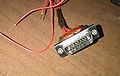
Fig 1a: DSub 26 connector
-
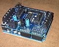
Fig 1b: Adafruit Motor Shield and Arduino
-
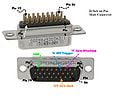
Fig 1c: D-Sub 26 Male Connector Pinout


On the Arduino board when a spectrum is meant to be measured it sends out a short TTL HIGH pulse to Pin 6 of the Dsub Connector. This triggers the spectrometer to Save Spectrum and store to computer memory.
A simple example of the TTL HIGH triggering for the spectrometer
//Matthew De Vuono
//May 30/2011
//Spectrometer triggering, TTL HIGH
void setup() {
// put your setup code here, to run once:
pinMode(7, OUTPUT);
Serial.begin(9600);
Serial.println("Sending Signal!");
Serial.println("Signal high");
digitalWrite(7, HIGH); // set the trigger on
delay(1000);
Serial.println("Signal low");
digitalWrite(7, LOW);
delay(3000);
Serial.println("Signal Sent");
delay(3000);
Serial.println("");
}
void loop()
{
}
In order to connect the Real time clock to the Arduino it is necessary to use the SDA and SCL pins. On most Arduino boards, SDA (data line) is on analog input pin 4, and SCL (clock line) is on analog input pin 5. On the Arduino Mega, SDA is digital pin 20 and SCL is 21. The Motor shield has these pins broken out for use since they are pins which are unused in the motor driver circuit.
Calibration and Verification[edit | edit source]
Use Spectrometer and light source calibration
This section needs to be cleaned up When the spectrometers were purchased they both came fully calibrated in the spectral response so that when they detected 300nm light the light was actually 300nm. However, only the one spectrometer was calibrated for absolute irradiance. This meant that we had to determine a way to calibrate this spectrometer without having to purchase thousands of dollars' worth of equipment. Since we had one calibrated unit we came up with a method ourselves.

It was possible to use our calibrated spectrometer to take detailed measurements of an ELH Halogen Projector bulb. These bulbs have a good spectral range and are consistent in terms of output over 24 hours of on time (losing <1%). We set the bulb up at a specific distance from the spectrometers sensor and allowed the bulb to reach steady-state in temperature and output. A full spectrum of the light was then taken from the bulb and we have now created an excel file with the spectral and Intensity data for this particular Halogen Light.
In order to ensure the bulb is at the same brightness here and over there in Cochabamba we are going to send the excel file, with the distance parameters, and send the halogen bulb. In Bolivia, we numerically integrated the spectrum sent, obtaining a result of 790.20 W/m^2
We used the Kipp&Zonen pyranometer [3] as a sensor, and with it's own factor of sensitivity (15.87 µV/W/m^2), we realized we had to get 12.55mV as an output, using the equivalence:
Radiation [W/m^2]= (Output [µV])/(Sensitivity cte [µV/W/m^2])
790.20 [W/m^2]= (Output [µV])/(15.87 [µV/W/m^2])
Output = 12553,17 [µV]]
Then, we fed the halogen bulb with a variac, connected to a 220-120V transformer, and, 251mm away, the pyranometer sensor conected to a multimeter, as seen in Picture 1. Waited for 20 minutes for the light to stabilize. When the intensity level required was reached (12.55mV), at 81,2 V ac from the variac, we swiched the pyranometer for the spectrometer (the extreme of the fiber connected to the cosine recepter) as seen in Picture 2. After that, we take the espectrum sent as a referece spectrum, and follow the steps of the SpectraSuite to get the Absolute Irradiance mode.

Once the data is taken and the graphs matched the calibration will be complete. Both curves, before calibration and after calibration are shown in figures 3a and 3b
-
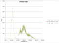
Fig 3a: Halogen Light in counts
-
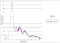
Fig 3b: Halogen light in uW/cm2/nm


Spectrometer Validation[edit | edit source]
In order to validate the results from the spectrometer, it was necessary to take measurements of some known light source. The best choice was to look at the actual out door sun, since it would best simulate the results we would be looking for. Initially, we got different results than what was expected as the spectrum plot didn't look as it should and
Parts list[edit | edit source]
| Part | Quantity | Description |
|---|---|---|
| Spectrometer | variable | Avantes AvaSpec-2048 Standard Fiber Optic Spectrometer
Avantes AvaSpec-NIR256/512-2.5TEC [4] OceanOptics USB4000 UV-VIS [5] |
| Stepper Motors | 2 | bipolar, 200 step [6] |
| Motor Driver board(MShield) | 1 | Adafruit Stepper Motor Driver Board[7] |
| Aluminum Square tube | 125" | 2.5"x1.5" |
| Aluminum plate 0.125" | 35" | 1/8" aluminum plate |
| 1" Aluminum Round Stock/1" polymer round stock | 1 | Turned down to size |
| Arduino Uno | 1 | The 'brains' of the system |
| DSUB 26 Connector | 1 | 26 pin connector Male [8] |
| Bolts and Nuts | 16 | 1/4-28 X 3" partially threaded bolts + nuts and washers [9] |
Operation Protocol[edit | edit source]
The operational protocol is very simple and needs only a computer and a sunny location.
Begin[edit | edit source]
The first thing to do is install the system in an area with access to a computer, power as well as internet access if possible. This location must be south facing if it is the northern hemisphere or north facing if it is the southern hemisphere. This is to ensure that the sensor will be able to view the sun all year long. It should be mounted in a location with a good view of the sky from the horizon up to above your head. A wall or roof top is ideal.
Location[edit | edit source]
Once the location is chosen it is important to ensure the weather-ability of the setup and that no snow or weather events will disturb it. It is going to have to stay in this position for at least a year undisturbed. This means checking the stepper Motors as well as the enclosure for the spectrometer as well as the humidity and temperature it will be subjected too.
Positioning[edit | edit source]
Now that the location is set up, it is important to calibrate the system in terms of headings and orientations. Initially make sure the system is facing southward and more importantly that the initial position of the shadowband and fibre coupler are set at the 0 degrees of elevation. This is to ensure that the consecutive measurements are all at a known level.
Stepper Motors[edit | edit source]
The stepper Motors must be connected to the Motor Shield
This table below refers to the Specific stepper listed above purchased from the Adafruit store. Different steppers may have different wire colour codes and coils. If you follow the directions below you can figure out your particular pinout.
| device | Stepper Number | Colour-terminal |
|---|---|---|
| Fibre Couple | 1 | Yellow,Red - M1
Green, Brown - M2 |
| ShadowBand | 2 | Yellow,Red - M3
Green, Brown - M4 |

These different colour wires represent the different coils of the stepper and as such must be connected in this particular manner. In order to ensure the wires are connected properly it is useful to measure the resistance between the different wire combinations. Two of those combinations will have the same resistance and the other two combinations will read infinite. It is these two pairs with the same resistance which should be connected to M1 and M2 respectively. Lastly, when the wires are connected it is important to attach the heat sinks onto the motor driver chips on the left and right side of the board. This site provides a better explanation.
The terminal M+ and GND must also be connected to a power source of no more than 12V 350mA. 5 V 800mA is sufficient to control 2 steppers. If a single power source is used it is necessary to keep the jumper attached to the PWR pins.
Software[edit | edit source]
The software used to operate the spectrometer is the Avasoft 7.5.3 USB software provided with the avantes spectrometer. After connecting to the spectrometer, the following set up tasks must be performed
- Link the VIS and IR spectrometers with the VIS spectrometer as master
- Merge the VIS and IR channels to ensure a smooth transition between spectrometers
- Cover light source and record a dark spectrum
- Subtract dark spectrum from data
- Set integration times to ensure that the raw readings (in counts) do not become saturated (above 66,000 counts). Currently the integration times are set to 47ms and 12 ms for the VIS and IR channels respectively.
- Enable excel output with an output delay of 0seconds
- Configure history channel functions to include the spectrum from the VIS and IR spectrometers
- Run history channels
When history channels are running with excel output enabled, Avasoft will start two instances of excel and begin to populate them with data from the spectrometer when triggered by the arduino controller. In order to periodically save these excel files, an external script was required which runs once daily to save the day's readings in excel. The script was written using AutoIt automation and complied as an executable. The script will activate the history channels window, close it to stop writing to the files, open each excel sheet individually and save it with a file name derived from the system time, close excel and re-enable history channel functions to prepare the system to collect data for the following day. The script used is shown below:
# include <GUIConstantsEx.au3>
# include <Date.au3>
# include <WindowsConstants.au3>

; Under Vista the Windows API "SetSystemTime" may be rejected due to system security
WinActivate("History Channel Functions")
sleep(2000)
send("!e")
sleep(1000)

$infFilePath="D:\Documents and Settings\rgauthier\Desktop\Spectrometer Dropbox\Dropbox\Dropbox Excel Data\Data\Infared"&@YEAR&"-"&@YDAY&"-"&@MON&"-"&@MDAY&"-"&@HOUR&"-"&@MIN&".xls"
$visFilePath="D:\Documents and Settings\rgauthier\Desktop\Spectrometer Dropbox\Dropbox\Dropbox Excel Data\Data\Visible"&@YEAR&"-"&@YDAY&"-"&@MON&"-"&@MDAY&"-"&@HOUR&"-"&@MIN&".xls"

Global Const $xlNormal = -4143 ;parameter to save as.xls
Global Const $iAccessMode = 1
Global Const $iConflictResolution = 2
Global $errcnt=0
$sType = $xlNormal ;sets the filetype to save

$oExcel = ObjGet("", "Excel.Application")
$errcnt=0
For $element In $oExcel.Application.Workbooks

 If $element.FullName = "Sheet1" Then
	 ;MsgBox(0,"",$element.FullName)
	 $element.SaveAs($infFilePath, $sType, Default, Default, Default, Default, $iAccessMode, $iConflictResolution)
	 $element.Close
 ElseIF 	$element.FullName = "Sheet2" Then
	 ;MsgBox(0,"",$element.FullName)
	 $element.SaveAs($visFilePath, $sType, Default, Default, Default, Default, $iAccessMode, $iConflictResolution)
	 $element.Close
 Else
	 $element.Activate
		 $errcnt=$errcnt+1
	 $errFilePath="D:\Documents and Settings\rgauthier\Desktop\Spectrometer Dropbox\Dropbox\Dropbox Excel Data\Data\Error"&@YEAR&"-"&@YDAY&"-"&@MON&"-"&@MDAY&"-"&@HOUR&"-"&@MIN&"-("&$errcnt&").xls"

	 $element.SaveAs($errFilePath, $sType, Default, Default, Default, Default, $iAccessMode, $iConflictResolution)
	 sleep(500)
	 $element.Close
 EndIf
Next
$oExcel.Application.Quit

sleep(1000)
WinActivate("AvaSoft")
sleep(1000)
send("!ahs")
Data[edit | edit source]
The data produced from this experiment consists of daily pairs of excel files with the naming convention:
[Infared or Visible][Year]-[Day of Year]-[Month]-[Day]-[Hour]-[Minute].xls
These datafiles have been combined into a unified database, which is distributed in.csv and.h5 file formats. In order to combine these datasets, the following processing steps were taken.
Import the visible and infrared datafiles as databases
Identify the angular position of the collecting head. The first reading is at 90 degrees from horizontal, the second is at 80, etc. to 0.
Set a multi index of date and position for each database
Join the visible and infrared channels on the date and position indicies, and append to the master database holding each day.
Carry out a dark correction for each day by subtracting the value from 1:00 am and 90 degrees each morning from each value in the day.
Time shift any data which was collected with an erronious time-stamp (data from Feb 25, 2013 to April 22, 2013 was lagging by 12 hours
Calulate the integrated energy for each hourly time stamp and position, and populate a Summary_info database with these values
For each hourly time stamp, poll pyranometer, meteorological and module performance data from the nearby OSOTF and append to the Summary info database
The full workflow for this processing was implemented in python using the pandas module, and the code is available in the project github and here: "http://bit.ly/OSOTF_Parser"
Data access and manipulation
The data is provided in a format which provides simplified access using the python pandas module. An Ipython console should be started, and the data can be loaded into active memory using the following commands:
 stre=pd.HDFStore(storepath')
 master=stre['Spec']
 Summary_info=stre['Summary']
 stre.close()
Where storepath is the location of the.h5 file containing the spectral data. This will load the data as a pandas dataframe with a two level multi-index: The top level being the date and hour and the second level being the position for each hour. Two dataframes are created, master holds the spectral information for each index location, and Summary_info contains the integrated spectral energy, and values collected from the nearby OSOTF.
In order to access as spectrum for a specific time and angle, the following python code can be used:
master.xs([datetime.datetime(year,month,day,hour),Position],level=['Date','Position'])
Where year, month, day, hour, and position must be defined by the user.
OpenSCAD Shadow Band code[edit | edit source]

//Customizable Shadow Band - to cast a shadow on solar radiation equipment so you can look at global and direct radiation
//Height of band
h=20;
// radius of band
r=50;
//Thickness of band
t= 5;
// Center extension width
w=10;
//Center extension hole size
e=2;

module shadowband (){
difference(){
union(){
rotate([0,90,0])cylinder(h = 2*r, r1 = w, r2 = w, center = true, $fn=250);
difference(){
cylinder(h = h, r1 = r, r2 = r, center = true, $fn=250);
cylinder(h = h+2, r1 = r-t, r2 = r-t, center = true, $fn=250);
translate([-r,0,-h/2-1])cube([2*r+2,r+1,h+2]);
}
}
rotate([0,90,0])cylinder(h = 2*r+2, r1 = e, r2 = e, center = true, $fn=250);
rotate([0,90,0])cylinder(h = 2*r-2*t, r1 = w+0.1, r2 = w+0.1, center = true, $fn=250);
}
}

shadowband ();
Related projects[edit | edit source]
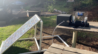
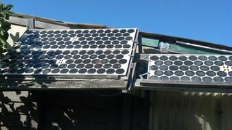
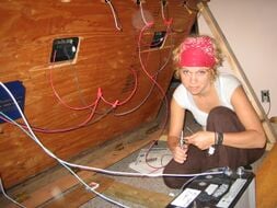
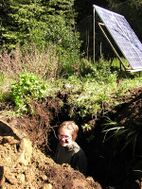
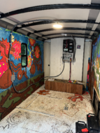
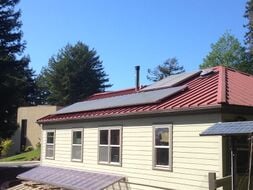
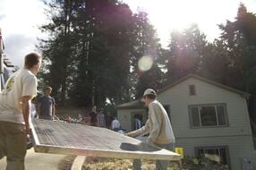
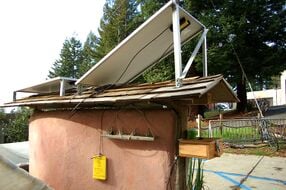
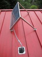
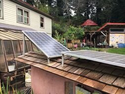
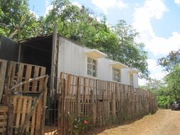
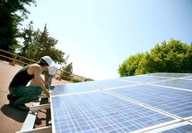
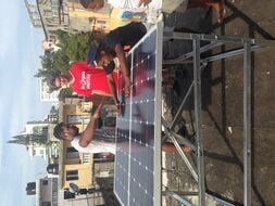
See also[edit | edit source]
- Installation of a variable-angle spectrometer system for monitoring diffuse and global solar radiation
- Spectrometer and light source calibration
- Download a customizable printable shadow band