
Solar Alone Multi-objective Advisor (SAMA)

| Type | |
|---|---|
| Authors | Seyyed Ali Sadat |
| Location | Canada |
| Status | In progress |
| Years | |
| Tools | Python |
| Uses | Sustainable development, renewable energy, energy policy, micro-grid design, educational purposes |
| Links | https://github.com/Sas1997/SAMA |
SAMA (Solar Alone Multi-objective Advisor) is an open-source (GNU GPL v3) energy system optimizer and analyzer mainly concentrated on stand-alone off-grid solar photovoltaic (PV)-based renewable energy systems (RES). SAMA allows for hybrid systems in locations that need a form of non-battery backup generation. Using SAMA, users can find the optimum size of a hybrid energy system for their property based on the electric load profile and meteorological data (irradiation, temperature and wind speed). Users can access economic data for their optimal energy system as a result of SAMA optimization and calculations. SAMA is developed in Python 3.9 using the NumPy, Numba, time, pandas, math, matplotlib and seaborn.
More information: Seyyed Ali Sadat, Jonathan Takahashi, Joshua M. Pearce, A Free and open-source microgrid optimization tool: SAMA the solar alone Multi-Objective Advisor, Energy Conversion and Management, 298, 2023, 117686, https://doi.org/10.1016/j.enconman.2023.117686. (Academia.edu)


Using SAMA
[edit | edit source]At the current version, SAMA is on the plain python code, but soon to be, an web tool and application exhibiting user interface will be designed for SAMA. To download SAMA newest version, please refer to its GitHub repository (Download all the files inside the SAMA V 1.01). Each part of software package back-end are described below. For comprehensive back-end discussion, please refer to SAMA user manual.
Watch this video discussing a case study in detail with SAMA and providing introductions how to use SAMA.
How to run SAMA
[edit | edit source]Step.1
Obtain the input data for simulations! To run SAMA, the user needs to define some data such as electrical load, temperature, irradiance, wind speed (if wind turbine is included in simulation), and costs. Hourly electrical load data for U.S different cities in a year (8760 values) can be downloaded from NREL library. Then in this file, extract the second column values from second row to the last value (8760 values) and replace them with first column of Eload.csv inside the content folder. Meteorological data (temperature, irradiance, wind speed) can be downloaded for any location in the world from NSRDB and be placed inside the content folder with METEO.csv name. Please note that when you download these data from NSRDB, the time interval should be 60 mins, and check to download DHI, DNI, Fill Flag, GHI, Ozone, Relative Humidity, Solar Zenith Angle, Surface Albedo, Pressure, Precipitable Water, Wind Direction, and Wind Speed (all meteorological the data). When defined electrical load and meteorological data or you decide how you want to define them, you need to define other inputs as discussed below completely (under Input_Data.py).
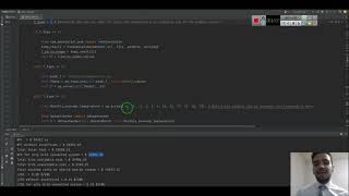
Step.2
Open the pso.py file in your preferred Python compiler and run it. For example, if user uses PyCharm environment, they just need to open pso.py in their PyCharm and run it! To run the code without error, user needs to make sure required Python packages (NumPy, Numba, time, pandas, math, matplotlib and seaborn) are installed prior to the run.
Enjoy!
Input_Data.py: The input data for simulations are defined inside this file.
[edit | edit source]# Optimization inputs
[edit | edit source]self.MaxIt=200: This parameter sets the maximum number of iterations or generations the PSO algorithm will run before terminating. The algorithm will stop once it reaches this limit.self.nPop = 50: This parameter determines the population size or swarm size. It specifies the number of particles in the swarm that will be used to explore the search space for an optimal solution.self.w = 1: This is the inertia weight, a coefficient that controls the balance between the particle's previous velocity and its cognitive and social components in updating its position. A higher value for 'w' means a greater emphasis on the particle's previous velocity.self.wdamp = 0.99: Inertia weight damping ratio. Over iterations, 'w' is typically reduced to decrease the impact of the previous velocity on particle movement. This parameter specifies the rate at which the inertia weight is reduced.self.c1 = 2: Personal learning coefficient, also known as cognitive coefficient. It controls the impact of a particle's best-known solution (individual experience) on its movement.self.c2 = 2: Global learning coefficient, also known as social coefficient. It controls the impact of the best-known solution within the entire swarm (collective experience) on a particle's movement.self.Run_Time = 1: This parameter sets the total number of runs in the simulation. In some cases, you might want to run the PSO algorithm multiple times and average the results to ensure robustness in finding the optimal solution.
# Lifetime and time definition
[edit | edit source]self.n = 25: This parameter represents the lifetime of the energy system in the simulations, specified in years.self.year = 2023: This parameter specifies the desired year within the simulation.
# Defining the electrical load
[edit | edit source]load_type is a variable that determines how you want to input the electrical load data. Depending on its value, different methods are used to define the load.
- If
load_typeis set to 1, the electrical load is loaded from a CSV file located at 'content/Eload.csv'. The data is read from the CSV file and stored in theself.Eloadarray. - If
load_typeis set to 2, the electrical load is defined as monthly hourly averages. Theself.Monthly_haverage_loadarray contains the hourly averages for each month, and thedataextenderfunction is used to extend this data into hourly values for the entire year. - If
load_typeis set to 3, the electrical load is defined as monthly daily averages. Theself.Monthly_daverage_loadarray contains the daily averages for each month, and the code converts these to hourly averages by dividing by 24. Thedataextenderfunction is then used to create hourly data for the entire year. - If
load_typeis set to 4, the electrical load is defined as monthly total load. Theself.Monthly_total_loadarray contains the total load for each month, and the code calculates monthly hourly averages based on the total load and the number of days in each month. Thedataextenderfunction is used to extend this data into hourly values for the entire year. - If
load_typeis set to 5, the electrical load is based on a generic load profile defined by the variableuser_defined_load. Thegeneric_loadfunction is used to generate hourly load values based on this generic profile. - If
load_typeis set to 6, the electrical load is defined as an annual hourly average, and all 8760 hours of the year are set to this average value. - If
load_typeis set to 7, the electrical load is defined as an annual daily average, and the code calculates the annual hourly average by dividing the daily average by 24. All 8760 hours of the year are set to this average value. - If
load_typeis set to 8, the electrical load is defined as an annual total load, and the code calculates the annual hourly average based on the total load and the number of days in each month. Thegeneric_loadfunction is used to generate hourly load values based on this annual total load. - If
load_typeis set to 9, a default generic load is used with a peak month definition of 'July or January'.
# Electrical load for previous year
[edit | edit source]It is defined similar to the electrical load discussed above. The electrical load for previous year is only needed for the situations we are going to calculate the grid costs and the monthly service charge scheme is tired rate structure. In other situations, users do not need to deal with this parameter.
# Irradiance definition
[edit | edit source]weather_url: This variable stores the URL or path to a weather data file in CSV format. The file is named 'METEO.csv' and likely contains weather-related data needed for simulating solar energy generation, such as solar irradiance, temperature, and other meteorological parameters. The specific content and format of the file depend on the simulation's requirements.azimuth: This variable specifies the azimuth angle in degrees, which represents the orientation of the photovoltaic (PV) modules. In this case, the azimuth is set to 180 degrees, which typically means that the PV modules are facing south.tilt: Thetiltvariable represents the tilt angle of the PV modules in degrees. A tilt angle determines the inclination of the PV panels from the horizontal plane. In this case, the tilt angle is set to 34 degrees.soiling: This variable stores the soiling loss percentage. Soiling losses refer to the reduction in energy generation due to dirt, dust, or other contaminants that accumulate on the PV modules over time.G_typeis a variable that determines how you want to input solar irradiance data. Depending on its value, different methods are used to define the irradiance data.- If
G_typeis set to 1, SAMA uses a built-in plane of array (POA) irradiance calculator based on the weather data stored in the CSV file specified byweather_url. Thetiltandazimuthangles of the PV modules, as well as a soiling loss percentage, are used as inputs for the simulation. The result is stored intemp_result, and the POA irradiance values are extracted from it and stored in theself.Garray. - If
G_typeis set to 2, the solar irradiance data is loaded from a CSV file located at 'content/Irradiance.csv'. The data is read from the CSV file and stored in theself.Garray. Please note that if you use this option, soiling losses will not be induced by SAMA itself.
- If
# Temperature definition
[edit | edit source]T_type is a variable that determines how you want to input temperature data for your simulation. Depending on its value, different methods are used to define the temperature data.
- If
T_typeis set to 1, the code imports therunSimulationfunction from thesam_monofacial_poamodule. This function is used to simulate temperature data based on the provided weather data, tilt, azimuth, and soiling parameters. The temperature data is extracted and stored in theself.Tarray. - If
T_typeis set to 2, the temperature data is loaded from a CSV file located at 'content/Temperature.csv'. The data is read from the CSV file and stored in theself.Tarray. - If
T_typeis set to 3, the temperature data is defined as monthly hourly averages. Theself.Monthly_average_temperaturearray contains the hourly averages for temperature for each month. Thedataextenderfunction is used to extend this data into hourly values for the entire year. - If
T_typeis set to 4, the temperature data is defined as an annual average temperature. Theself.Annual_average_temperaturevariable is set to desired annual average, and all 8760 hours of the year are set to this average temperature.
# Wind speed definition
[edit | edit source]WS_type is a variable that determines how you want to input wind speed data for your simulation. Depending on its value, different methods are used to define the wind speed data.
- If
WS_typeis set to 1, the code imports therunSimulationfunction from thesam_monofacial_poamodule. This function is used to simulate wind speed data based on the provided weather data, tilt, azimuth, and soiling parameters. The wind speed data is extracted and stored in theself.Vwarray. - If
WS_typeis set to 2, the wind speed data is loaded from a CSV file located at 'content/WSPEED.csv'. The data is read from the CSV file and stored in theself.Vwarray. - If
WS_typeis set to 3, the wind speed data is defined as monthly hourly averages. Theself.Monthly_average_windspeedarray contains the hourly averages for wind speed for each month. Thedataextenderfunction is used to extend this data into hourly values for the entire year. - If
WS_typeis set to 4, the wind speed data is defined as an annual average wind speed. Theself.Annual_average_windspeedvariable is set to desired annual wind speed, and all 8760 hours of the year are set to this average wind speed.
# Type of systems included in simulations
[edit | edit source]self.PV: This indicates that a photovoltaic (PV) system is included in the simulation (with a value of 1) or not (with a value of 0).self.WT:This indicates that a a wind turbine (WT) system is included in the simulation (with a value of 1) or not (with a value of 0).self.DG: This indicates that a diesel generator (DG) system is included in the simulation (with a value of 1) or not (with a value of 0).self.Bat: This indicates that a battery system in the simulation (with a value of 1) or not (with a value of 0).self.Grid = 1: This indicates if grid interconnection is included in the simulation, indicated by a value of 1. If you want to simulate a off-grid system without a grid connection, you would set this to 0.self.NEM = 1: This parameter is related to net metering. If set to 1, it means that compensation in the net metering scheme is provided as credits, not as monetary compensation. In this case, yearly credits will be reconciled after 12 months.
# Constraints
[edit | edit source]self.LPSP_max_rate: This parameter represents the maximum acceptable loss of power supply probability (LPSP) in percentage form.self.RE_min_rate: This parameter represents the minimum required renewable energy (RE) capacity as a percentage.
# Multi-objective optimization
[edit | edit source]If self.EM = 0the objective for optimization is only NPC while if self.EM = 1the objectives for optimization are NPC and levelized emission (LE).
# Rated capacity (DO NOT CHANGE)
[edit | edit source]# PV technical parameters
[edit | edit source]self.fpv = 0.9: This parameter represents the derating factor for the PV module, expressed as a percentage (90%). It accounts for efficiency losses and performance degradation in the PV module over time.self.Tcof = 0: The temperature coefficient for the PV module, expressed as a percentage per degree Celsius (%/°C). It quantifies how the PV module's performance is affected by changes in temperature.self.Tref = 25: The reference temperature at standard test conditions for the PV module, typically 25°C. This is used to normalize the module's performance data.self.Tc_noct = 45: The nominal operating cell temperature for the PV module. It represents the temperature of the PV cells during operation under specified conditions.self.Ta_noct = 20: The ambient temperature used for determining the nominal operating cell temperature. It is typically lower than the cell temperature due to the module's heat dissipation.self.G_noct = 800: The solar irradiance at the nominal operating cell temperature. It represents the solar radiation level used to calculate the NOCT.self.gama = 0.9: A parameter related to the conversion efficiency of the PV module.self.n_PV = 0.2182: The efficiency of the PV module. This value likely represents the efficiency of converting incident solar energy into electrical energy.self.Gref = 1000: The reference solar irradiance level, typically 1000 watts per square meter (W/m^2), used for normalizing PV module performance data.self.L_PV = 25: The lifetime of the PV module in years. This parameter defines the expected operational lifespan of the PV module in your simulation.
# WT technical parameters
[edit | edit source]self.h_hub = 17: This parameter represents the hub height of the wind turbine in meters. It specifies the height at which the wind turbine is mounted, and it is an important factor affecting wind energy capture.self.h0 = 43.6: The anemometer height in meters. Anemometer height is the height at which wind speed measurements are taken and is typically used to calculate wind shear.self.nw = 1: The electrical efficiency of the wind turbine, expressed as a decimal. It indicates the fraction of the wind's kinetic energy that is converted into electrical energy.self.v_cut_out = 25: The cut-out speed in meters per second (m/s). When the wind speed exceeds this value, the wind turbine is typically shut down or "cut out" to prevent damage.self.v_cut_in = 2.5: The cut-in speed in meters per second (m/s). It is the wind speed at which the wind turbine starts operating and generating electricity.self.v_rated = 9.5: The rated speed of the wind turbine in meters per second (m/s). This is the wind speed at which the wind turbine generates its maximum rated power.self.alfa_wind_turbine = 0.14: The coefficient of friction. This parameter is used to model the effects of friction on the wind turbine's performance. The value may vary depending on wind conditions, with lower values for extreme wind conditions and higher values for normal wind conditions.self.L_WT = 20: The lifetime of the wind turbine in years. This parameter defines the expected operational lifespan of the wind turbine in your simulation.
# DG technical parameters
[edit | edit source]self.LR_DG = 0.25: This parameter represents the minimum load ratio for the DG system, expressed as a percentage (%). It specifies the minimum load that the DG can operate at efficiently.- Diesel Generator Fuel Curve:
self.a = 0.2730: The coefficient 'a' in liters per hour per kilowatt (L/hr/kW) of DG output. It is used to model the DG's fuel consumption rate as a function of its output power.self.b = 0.0330: The coefficient 'b' in liters per hour per kilowatt (L/hr/kW) of the DG's rated power. It is used in the fuel consumption model.
self.TL_DG = 24000: The lifetime of the diesel generator in hours. This parameter defines the expected operational lifespan of the DG in your simulation.- Emissions produced in gr by DG for liter of fuel consumed
self.CO2: The emission level of carbon dioxide (CO2) in grams per liter (g/L) of fuel. CO2 is a greenhouse gas and a major contributor to global warming.self.CO: The emission level of carbon monoxide (CO) in grams per liter (g/L) of fuel. Carbon monoxide is a harmful air pollutant that can have adverse effects on air quality and human health.self.NOx: The emission level of nitrogen oxides (NOx) in grams per liter (g/L) of fuel. NOx includes nitrogen dioxide (NO2) and nitric oxide (NO), which are harmful air pollutants and contribute to smog and acid rain.self.SO2: The emission level of sulfur dioxide (SO2) in grams per liter (g/L) of fuel. SO2 is a harmful air pollutant that can lead to respiratory problems and contribute to acid rain.
# Battery technical parameters
[edit | edit source]self.SOC_min = 0.2: The minimum state of charge (SOC) of the battery. SOC represents the fraction of the battery's capacity that is currently used, and this parameter sets the minimum allowed SOC.self.SOC_max = 1: The maximum SOC of the battery, representing the fully charged state. It is typically set to 1 for full capacity.self.SOC_initial = 0.5: The initial SOC of the battery when the simulation starts.self.Q_lifetime = 8000: The lifetime capacity of the battery, expressed in kilowatt-hours (kWh). This value represents the total energy that the battery is capable of storing over its lifetime.self.self_discharge_rate = 0: The hourly self-discharge rate of the battery, which is a measure of how much energy is lost over time due to self-discharge. A rate of 0 indicates no self-discharge.self.alfa_battery = 1: The storage's maximum charge rate, given as a ratio of charge current to the battery's capacity (A/Ah). This parameter is related to the battery's charge and discharge characteristics.self.c = 0.403: The storage capacity ratio, which is a unitless parameter related to the battery's capacity and performance.self.k = 0.827: The storage rate constant, given in units of per hour (h⁻¹). This parameter influences the rate at which the battery can charge or discharge.self.Imax = 16.7: The battery's maximum charge current, expressed in amperes (A).self.Vnom = 12: The battery's nominal voltage, specified in volts (V).self.ef_bat = 0.8: The round-trip efficiency of the battery. This parameter represents the efficiency of charging and discharging the battery.self.L_B = 7.5: The lifetime of the battery in years. This parameter defines the expected operational lifespan of the battery in your simulation.
# Inverter
[edit | edit source]self.n_I: This parameter represents the efficiency of the inverter. It is expressed as a decimal and indicates the fraction of electrical power that is converted from direct current (DC) to alternating current (AC) by the inverter.self.L_I: The lifetime of the inverter in years. This parameter defines the expected operational lifespan of the inverter in your simulation.self.DC_AC_ratio: The maximum acceptable DC to AC ratio. This parameter specifies the maximum ratio of DC power (input) to AC power (output) that the inverter can handle efficiently.
# Charger
[edit | edit source]The parameter self.L_CH is related to the charge controller used in your simulation and represents the lifetime of the charger in years.
# Economic inputs
[edit | edit source]self.n_ir_rate: The nominal discount rate, expressed as a percentage. It represents the rate at which future cash flows are discounted to determine their present value.self.e_ir_rate: The expected inflation rate, expressed as a percentage. It accounts for the expected rate of price inflation over time..self.Budget: The budget or limit on the total capital cost for the project, expressed in dollars. This parameter sets a constraint on the total capital expenditure.self.Tax_rate: The equipment sales tax rate, expressed as a percentage. It represents the percentage of tax applied to the purchase of equipment.self.RE_incentives_rate: The federal tax credit rate for renewable energy incentives, expressed as a percentage. This parameter represents the percentage of federal tax credit that can be applied to the project.
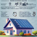
# Top down pricing inputs
[edit | edit source]self.Pricing_method: This parameter is used to determine the pricing method. If it is set to "1", it refers to the top-down pricing method and "2" refers to bottom up pricing method. In the top-down pricing method, the PV system costs are broke down based on NREL PV cost benchmarks. In bottom up pricing method, users need to define each equipment cost in detail (Capital, replacement and maintenance).
For top-down pricing method:
Total_PV_price = 2950: The total price for PV system (PV+inverter+engineering costs) in $ per kW. This is the initial cost of the PV system.- Rather than PV and inverter, users need to define costs in $ per kW for other system components and $ per kWh for battery, such as wind turbines (WT), diesel generators (DG), batteries (B), and chargers (CH), including their capital costs, replacement costs, and operation and maintenance (O&M) costs. These costs are based on the capital costs and replacement costs in dollars.
- Some components, like the diesel generator (DG) fuel cost, also consider yearly escalation or reduction rates in fuel cost.
top-down pricing allows you to model the initial and ongoing costs of the various components of your energy system. The top-down pricing method starts with the total cost and allocates it to individual components based on predefined relationships and cost factors.
# Bottom up pricing inputs
[edit | edit source]This approach specifies the costs associated with individual components of the energy system. Here's a breakdown of the pricing information for each component:
- Engineering Costs (Per/kW):
self.Installation_cost = 160: The cost of installation per kilowatt (kW) of installed capacity.self.Overhead = 260: Overhead costs per kW.self.Sales_and_marketing = 400: Sales and marketing costs per kW.self.Permiting_and_Inspection = 210: Permitting and inspection costs per kW.self.Electrical_BoS = 370: Electrical balance of system (BoS) costs per kW.self.Structural_BoS = 160: Structural BoS costs per kW.self.Supply_Chain_costs = 0: Supply chain costs per kW.self.Profit_costs = 340: Profit costs per kW.self.Sales_tax = 80: Sales tax per kW.self.Engineering_Costs: The total engineering costs per kW, calculated as the sum of all the individual cost components.
- PV (Photovoltaic) System:
self.C_PV = 2510: The capital cost of the PV system per kW.self.R_PV = 2510: The replacement cost of PV modules per kW.self.MO_PV = 28.12: The annual O&M cost per kW.
- Inverter:
self.C_I = 440: The capital cost of the inverter per kW.self.R_I = 440: The replacement cost of the inverter per kW.self.MO_I = 3: The annual O&M cost per kW.
- Wind Turbine (WT) System:
self.C_WT = 1200: The capital cost of the wind turbine system per kW.self.R_WT = 1200: The replacement cost of wind turbines per kW.self.MO_WT = 40: The annual O&M cost per kW.
- Diesel Generator (DG) System:
self.C_DG = 240.45: The capital cost of the diesel generator system per kW.self.R_DG = 240.45: The replacement cost of the diesel generator per kW.self.MO_DG = 0.064: The annual O&M cost per operating hour.self.C_fuel = 1.39: The fuel cost per liter (L) for the DG system.self.C_fuel_adj_rate = 2: The yearly escalation or reduction rate of DG fuel costs.self.C_fuel_adj = self.C_fuel_adj_rate / 100: The rate converted to a decimal form.
- Battery System:
self.C_B = 458.06: The capital cost of the battery system per kWh.self.R_B = 458.06: The replacement cost of the battery per kWh.self.MO_B = 10: The annual maintenance cost per kWh.
- Charger:
self.C_CH = 149.99 * (1 + self.r_Sales_tax): The capital cost of the charger. The sales tax is applied to the cost.self.R_CH = 149.99 * (1 + self.r_Sales_tax): The replacement cost of the charger. The sales tax is applied to the cost.self.MO_CH = 0 * (1 + self.r_Sales_tax): The annual O&M cost for the charger. The sales tax is applied to the cost.
# Defining prices for electric utilities
[edit | edit source]self.rateStructure: This parameter specifies the hourly rate structure for electricity prices. The values below for this parameter show the corresponding rate structure. Users can choose whichever fits them best.
1 = flat rate
2 = seasonal rate
3 = monthly rate
4 = tiered rate
5 = seasonal tiered rate
6 = monthly tiered rate
7 = time of use rate
self.Annual_expenses: This parameter represents any annual expenses in dollars associated with the grid.self.Grid_sale_tax_rate: This parameter represents the sales tax percentage applied to grid electricity prices.self.Grid_Tax_amount: This parameter represents a grid tax applied in kilowatt-hours (kWh).self.Grid_escalation_rate: This parameter defines the yearly escalation rate for grid electricity prices, expressed as a percentage.self.Grid_credit: This parameter represents any credits offered by the grid to users in dollars.self.NEM_fee: This parameter represents any one-time setup fee for net metering.
# Monthly service charge (buying prices)
[edit | edit source]self.Monthly_fixed_charge_system: This parameter specifies the type of monthly fixed charge structure. If It is set to "1" indicating a flat monthly rate over the year and if it is "2", indicating a tiered structure for monthly charges. The self.SC_flatis the monthly flat charge in structure 1.
Structure 2 includes tier-specific service charge values and limits for each tier:
self.SC_1 = 2.30: The service charge for tier 1 in $.
self.Limit_SC_1 = 350: The limit for tier 1 in kWh.
self.SC_2 = 7.9: The service charge for tier 2 in $.
self.Limit_SC_2 = 1050: The limit for tier 2 in kWh.
self.SC_3 = 22.70: The service charge for tier 3 in $.
self.Limit_SC_3 = 1501: The limit for tier 3 in kWh.
self.SC_4 = 22.70: The service charge for tier 4 in $.
# Utility hourly charges (buying prices)
How to define hourly charges for grid:
- Set Rate Structure:
- Determine the rate structure you want to simulate. The rate structure is specified by the
self.rateStructurevariable.
- Determine the rate structure you want to simulate. The rate structure is specified by the
- Configure Rate Parameters:
- Depending on the chosen rate structure, configure the rate parameters accordingly:
- For flat rate, set the
self.flatPrice. - For seasonal rate, specify seasonal prices in
self.seasonalPricesand define the season inself.season. - For monthly rate, provide monthly prices in
self.monthlyPrices. - For tiered rate, set tiered prices in
self.tieredPricesand tier maximums inself.tierMax. - For seasonal tiered rate, provide seasonal tiered prices and maximums in
self.seasonalTieredPricesandself.seasonalTierMax. - For monthly tiered rate, configure monthly tiered prices and maximums in
self.monthlyTieredPricesandself.monthlyTierLimits. - For time-of-use rate, specify on-peak, mid-peak, and off-peak prices, special hours for holidays, and the season in
self.onPrice,self.midPrice,self.offPrice,self.holidays,self.season, and the time-of-use hours inself.onHoursandself.midHours.
- For flat rate, set the
- Depending on the chosen rate structure, configure the rate parameters accordingly:
# Sell back prices to the grid
[edit | edit source]How to define hourly sell back prices to the grid:
- Set Sell Structure:
- Determine the structure for selling electricity to the grid by setting the
self.sellStructurevariable. You can choose from three options:1: Flat rate for selling electricity back to the grid.2: Monthly rate for selling electricity back to the grid.3: Selling electricity back to the grid at the same rate you buy it.
- Determine the structure for selling electricity to the grid by setting the
- Configure Sell Rates:
- Depending on the chosen sell structure, configure the sell rates accordingly:
- For flat rate (sellStructure = 1), set the desired flat sell rate in the
self.Csellvariable. - For monthly rate (sellStructure = 2), provide an array of monthly sell prices in
self.monthlysellprices. The array should contain 12 values, one for each month. - For selling at the same rate as you buy (sellStructure = 3), you can set
self.Cselltoself.Cbuy. This means you will sell electricity back to the grid at the same rate you buy it.
- For flat rate (sellStructure = 1), set the desired flat sell rate in the
- Depending on the chosen sell structure, configure the sell rates accordingly:
# Grid emission information
[edit | edit source]self.E_CO2: The emission level of carbon dioxide (CO2) in kg per kWh of electricity bought from grid.self.E_NOx: The emission level of nitrogen oxides (NOx) in kg per kWh of electricity bought from grid.self.E_SO2: The emission level of sulfur dioxide (SO2) in kg per kWh of electricity bought from grid.
# Constraints for buying/selling from/to grid
[edit | edit source]These lines of code set constraints for buying and selling electricity from/to the grid:
self.Pbuy_max: This represents the maximum amount of electricity that can be bought from the grid in each hour in kW (Maximum buying capacity).self.Psell_max: This represents the maximum amount of electricity that can be sold to the grid in each hour in kW (Maximum selling capacity).
swarm.py: In this file, the optimization algorithm which particle swarm optimizer (PSO) code is written.
[edit | edit source]Fitness.py: The file including cost calculations and fitness function for optimizer.
[edit | edit source]EMS.py: Energy management strategy has been implemented inside this file.
[edit | edit source]Battery_Model.py: Chemical battery models are defined inside this file.
[edit | edit source]calcFlatRate.py, calcMonthlyRate.py, calcMonthlyTieredRate.py, calcSeasonalRate.py, calcSeasonalTieredRate.py, calcTieredRate.py, and calcTouRate.py: Electric Utility billing schemes are defined in the files above.
[edit | edit source]See Also
[edit | edit source]See Also
[edit source]

- A Review of Phase-Change Material-Based Thermal Batteries for Sustainable Energy Storage of Solar Photovoltaic Systems Coupled to Heat Pumps in the Building Sector
- Decarbonization of Residential Houses in Northern Climates: Traditional vs Fully Electrified Approaches in Ontario Canada
| Authors | |
|---|---|
| License | CC-BY-SA-4.0 |
| Cite as | Seyyed Ali Sadat (2023–2026). "Solar Alone Multi-objective Advisor (SAMA)". Appropedia. Retrieved July 12, 2026. |