
What Is OpenFOAM?[edit | edit source]
OpenFOAM is the leading, open source CFD software which is very well known across the world and across a wide range of engineers and researchers. Being free and open source, and also having the ability to solve almost anything from complex fluid flow structures and heat transfer to combustion and chemical reactions, have made OpenFOAM one of the most popular softwares among mechanical engineers.
This tutorial aims to give you a brief insight of how to download and install the software, how it works, how to use the tutorial projects and primary codes, and how to modify the primary codes to simulate a complicated fluid flow structure.
How to Download and Install OpenFOAM?[edit | edit source]
Preferably, the best way to use this software is to install it on Linux operating systems; and the most preferred version of Linux to run OpenFOAM is the last version of Ubuntu at the time. For those who use different versions of Windows or Mac as an operating system on their laptops or computers, the easiest way to use OpenFOAM will be installing a virtual machine instead of using two different operating systems on one computer.
The following link navigates you to the download page of ORACLE Virtual Machine website, where you can find direct download links for ORACLE VM installer packages for different operating systems: https://www.virtualbox.org/wiki/Downloads
After installing the Virtual Machine on your computer, then you can easily install Ubuntu operating system on the virtual machine using the following instructions:
How to run an Ubuntu Desktop virtual machine using VirtualBox
How to Install Ubuntu on VirtualBox in Windows
How to Install Ubuntu on a MacOS using VirtualBox
Now everything is ready to download and install the OpenFOAM software. The easiest way to download and install OpenFOAM is to open a terminal in Ubuntu OS and copy and paste the following commands:
- To add OpenFOAM to the list of software repositories to search and download the OpenFOAM software (This stage only needs to be done once for every computer) :
sudo sh -c "wget -O - https://dl.openfoam.org/gpg.key > /etc/apt/trusted.gpg.d/openfoam.asc"
sudo add-apt-repository http://dl.openfoam.org/ubuntu
2. In order to update the "apt" package list to download OpenFOAM :
sudo apt-get update
3. To install the last version of OpenFOAM (this code refers to OpenFOAM version 10 and the newest version of ParaView) :
sudo apt-get -y install openfoam10
4. Because the OpenFOAM packages gets periodically recompiled into a new pack, you should type the following lines to patch your software :
sudo apt-get update
sudo apt-get upgrade
The installation process is finished and the OpenFOAM software is ready to run. For any possible installation problems, you can refer to common installation problems.
How to Run Our First Simulation in OpenFOAM[edit | edit source]
First, we should know how OpenFOAM works. After finishing the installation process, you can find a folder named OpenFOAM in the installation address which contains every code and file you need to run your simulations. As the most important folders, the “applications” and “tutorials” respectively contain all of the source codes for different solvers and numerous examples of simple and complex case studies in fluid dynamics, heat transfer, combustion and etc. The main way to simulate every complex case study with OpenFOAM is to find the most similar tutorial to our main problem and modify the codes to create the closest model to our main case study, which will be discussed later. But for now, the easiest way to run our first simulation with OpenFOAM is to use one of the tutorials available.
As a basic problem to learn how to do the case setup, apply initial values, set up the boundary conditions and mesh, as well as simulate the problem, we will use the elbow tutorial which can be found in the directory of “OpenFOAM/tutorials/incompressible/icoFoam/elbow”. It is important to note that the icoFoam solver is one of the basic transient solvers for Newtonian, incompressible, laminar fluid flows. The following picture shows how an OpenFOAM case study looks like.
.png)
The “zero” folder contains the initial conditions of the simulation and in this case, there are only two files named “P” and “U” representing the initial pressure and velocity fields respectively. The “constant” folder contains only the “physicalproerties” file defining the magnitude of the kinematic viscosity. In the “system” folder you will normally find files for controlling the simulation process, which gives you control over the solution scheme, time steps, and discretization schemes. Last but not least, the “elbow.msh” file defines the solution domain of the case study (geometry and mesh). For the first simulation, we do not need to make any changes in these files, but we will discuss how to do that later in the next simulations.
After going through the above-mentioned files (and applying any necessary changes), our case study is ready to be simulated. In order to start the simulation, open the tutorial’s path using a terminal and then call {fluentMeshToFoam “name of the mesh file”} command to create the geometry and apply mesh on the domain. Now that the geometry and mesh have been created, you can call {paraview &} command to open paraview software to have a visual export of what you have done so far. After paraview software opens, go through the path {File/Open/(the tutorial folder)/system/controldict}, open “controldict” file, and then press the “Apply” button. The geometry and mesh will be projected as follows:
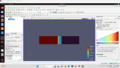
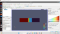
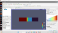
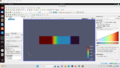
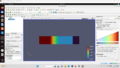
Now that we have set up the case and imported the mesh, it is time to run the simulation and see the results. To run the simulation, go back to the terminal and type {icoFoam} and press Enter, and the simulation will be running. After the simulation stops, open paraview software and import your solution through {File/Open//(the tutorial folder)/system/controldict} directory and then press “Apply” button. The solution is ready now, and you can export different types of contours and other graphical results from paraview software as follows:
.png)
.png)
.png)
To receive more accurate results and contours, sometimes you need to apply a larger number of cells to the solution domain. To do so, after calling your mesh file using {fluentMeshToFoam} command, you can increase the number of cells under the same meshing strategy by using {refineMesh -overwrite} which will increase the number of cells by reducing the cell size and will overwrite the new mesh file.
When the refinement is done, you will see a report of the refinement process in the terminal, which offers information about how the refinement has been applied and details of the new refined mesh. By writing {icoFoam} command in the terminal, the simulation will start running using the new mesh file. The following pictures show the cell structure and the results of the simulation under the new refined mesh file:


How to Create a Solution Domain with blockMesh?[edit | edit source]
In this part of the tutorial, we will learn how to create our own geometry and then apply cells to solve our problem using any related solver. As the first step, similar to the previous parts of the tutorial, we will choose the most similar tutorial to our problem. In every tutorial in the OpenFOAM directory, there is a folder named system containing blockMeshDict, controlDict, fvSchemes, and fvSolution. The blockMeshDict file contains all of the information about the geometry and mesh of the solution domain.
To make it easier to understand, we pick a tutorial as a reference to modify. As a simple example, the "rhoPimpleFoam/laminar/forwardstep" is suitable, which is a laminar compressible sonic/supersonic solver.
In order to modify the domain of the problem, some changes have to be applied to the blockMeshDict file. The most important sections inside the blockMeshDict file are vertices, blocks, and boundary. vertices are the location of nodes that represent the corners of the geometry, and any of the three numbers inside the bracket represents the distance of the node from the origin in X, Y, and Z directions. For example, the vertices of "rhoPimpleFoam/laminar/forwardstep" solver is as follows:
vertices
(
(0 0 -0.05)
(0.6 0 -0.05)
(0 0.2 -0.05)
(0.6 0.2 -0.05)
(3 0.2 -0.05)
(0 1 -0.05)
(0.6 1 -0.05)
(3 1 -0.05)
(0 0 0.05)
(0.6 0 0.05)
(0 0.2 0.05)
(0.6 0.2 0.05)
(3 0.2 0.05)
(0 1 0.05)
(0.6 1 0.05)
(3 1 0.05)
);
After defining the geometry by vertices, we will apply the mesh to the geometry using the "blocks" section. In this section, you will need to write something similar to the following lines:
hex (0 1 3 2 8 9 11 10) (25 10 1) simpleGrading (1 1 1)
hex (2 3 6 5 10 11 14 13) (25 40 1) simpleGrading (1 1 1)
hex (3 4 7 6 11 12 15 14) (100 40 1) simpleGrading (1 1 1)
Every geometry can be divided into simpler geometries which are connected to each other. The first bracket in each line contains the number of vertices that make a block, a part of the main geometry, if connect to each other. the second bracket shows the number of cells on the edges of each block in the X, Y, and Z directions respectively. and finally, the last bracket can be used whenever biased mesh is needed. By changing the third bracket, the concentration of the cells on the edges will change.
The next important part of the blockMeshDict file is the boundary section. In this section, the location and the type of boundaries will be defined. As an example, the boundary part of the mentioned tutorial is presented:
boundary
(
inlet
{
type patch;
faces
(
(0 8 10 2)
(2 10 13 5)
);
}
outlet
{
type patch;
faces
(
(4 7 15 12)
);
}
bottom
{
type symmetryPlane;
faces
(
(0 1 9 8)
);
}
top
{
type symmetryPlane;
faces
(
(5 13 14 6)
(6 14 15 7)
);
}
obstacle
{
type wall;
faces
(
(1 3 11 9)
(3 4 12 11)
);
}
);
The "patch" is the type of boundary condition that we mostly use for inlet and outlet boundaries. Whenever our geometry is symmetric and can be mirrored on one of the boundaries, we will use the "symmetryplane" as the boundary type. Similarly, when we need to apply the no-slip boundary condition to a surface, we allocate "wall" boundary type to the edge or surface. In addition, another important principle here is to use Right-Hand Rule to introduce the boundary nodes, which has a direct impact on the direction of the normal vector of the boundary.
After defining the geometry and mesh by modifying the blockMeshDict file, we will execute the "blockMesh" command, which produces the geometry and mesh. By opening the "boundary" file in "rhoPimpleFoam/laminar/forwardstep/constant/polymesh" directory, we can see the exact boundary conditions applied on every face of the geometry according to what we defined in the "blockMeshDict" file.
The Final step is to run the solver and extract the results using Paraview software. The results of the mentioned tutorial are shown below to make a better understanding of what we defined during this session.


Grid Convergence Study[edit | edit source]
In this section, we are going to check the influence of grid size on the results of the simulation. To do so, a shock tube problem is selected to be solved by the "rhoCentralFoam" solver, which is a compressible, single-phase, transient, non-isothermal solver with the ability to solve both transient and laminar fluid flows. The geometry of this problem is a rectangular duct with a width and depth of 2 meters and a length of 10 meters. Also, the problem is one-dimensional and the flow regime is considered to be laminar, and the fluid is an ideal gas. The problem has been considered transient and solved for 7 ms.
To compare the results of a low-resolution grid with a high-resolution one, according to the previous part of this tutorial, two rectangular tubes with 100 and 1000 cells in X direction, and only one cell in Y and Z direction are defined separately.
.png)
.png)
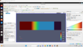
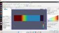
In order to simulate the shock tube conditions, we allocate two different pressure magnitudes namely 0 and 100000 Pa to first and second half of the rectangular duct respectively. To do so, we modify the "setFieldsDict" file as follows:
/*--------------------------------*- C++ -*----------------------------------*\
========= |
\\ / F ield | OpenFOAM: The Open Source CFD Toolbox
\\ / O peration | Website: https://openfoam.org
\\ / A nd | Version: 10
\\/ M anipulation |
\*---------------------------------------------------------------------------*/
FoamFile
{
format ascii;
class dictionary;
location "system";
object setFieldsDict;
}
// * * * * * * * * * * * * * * * * * * * * * * * * * * * * * * * * * * * * * //
defaultFieldValues
(
volVectorFieldValue U (0 0 0)
volScalarFieldValue T 348.432
volScalarFieldValue p 0
);
regions
(
boxToCell
{
box (0 -1 -1) (5 1 1);
fieldValues
(
volScalarFieldValue T 278.746
volScalarFieldValue p 100000
);
}
);
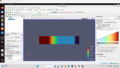
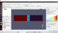
Then we should execute the "setFields" command in the terminal to initialize the parameters in the solution domain. The next step would be solving the problem using the "rhoCentralFoam" for the two different mesh strategies. After executing the "rhoCentralFoam" command in the terminal, the final results will be accessible through the Paraview software as follows:
- The pressure contour of the shock tube with 100 cells for each time step
-
-
-
-
-
-
-
.png)
.png)
.png)
.png)
.png)
.png)
.png)
- The pressure contour of the shock tube with 1000 cells for each time step
-
-
-
-
-
-
-
.png)
.png)
.png)
.png)
.png)
.png)
.png)
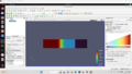
To better understand the difference between the above galleries, let's take a look at the physics of a shock tube. By initializing and applying two different pressure magnitudes on two different zones of the tube, we have made high-pressure and low-pressure zones which are separated from each other by an imaginary barrier. when the transient simulation starts, the imaginary barrier disappears and the fluid flows toward the low-pressure zone and simulates a shock in the tube. The difference between high-resolution and low-resolution grids can easily be seen by comparing the above pictures. The low-resolution grid simulates the shock (the transition zone between high-pressure and low-pressure parts) within a few numbers of meshes (control volumes) which means a distance in centimeter scale which is not physically accurate, while the high-resolution grid models the shock in less than one millimeter of the tube. This simple example shows the amount of precision that a high-quality mesh can add to the simulation. Hence, the first step in numerical simulations would be checking the accuracy of the grid by applying the grid independence procedure.
For those who need to know, the grid independence check means to make sure that the grid is fine enough so that any slight increase in the number of meshes will not change the results of the simulation. In other words, the grid is precise enough that the results of the simulation are independent of the mesh size.
Combination of Tutorials[edit | edit source]
As I mentioned before, we almost always make our projects by combining and modifying different tutorials. In this section, in order to gain a better understanding of the concept of diffusion and convection terms of the energy equation, we will combine and then modify "scalarTransportFoam" solver and "forwardStep" tutorial that can be find in "OpenFoam-10/tutorials/basic" and "OpenFoam-10/tutorials/compressible/rhoPimpleFoam/laminar" directories respectively.
The aim of this session is to solve the solution domain of "forwardStep" problem using "scalarTransportFoam" solver to show the role of different terms in the energy equation. The first step is to copy the "forwardStep" folder to the solver's directory. Then we should apply some modifications to the "forwardStep" problem to be solvable by the new solver. To do so, we compare the "forwardStep" case to one of the tutorials available in the solver's directory.
Starting with the "0" folder, our solver only needs temperature and velocity fields to solve the energy equation in the fluid flow, so we will delete the "P" (pressure) file from the "forwardStep" problem. In the "constant" folder of the "forwardStep" problem, there is a "momentumTransport" file which is not necessary for the solver and it is better to be deleted. There is also a "physicalProperties" file which must be replaced by the same file from the solver's directory because the solver needs only the diffusivity to solve the energy equation. The last and most important folder, system, contains three files namely "controlDict", "fvSchemes", and "fvSolution" that must be replaced in the "forwardStep" case. "controlDict" file controls the start and stop time of the solution plus the number and the size of time steps. The "fvScheme" file defines different discretization methods and numerical schemes for terms such as derivatives that appear in the equation, and the "fvSolution" file contains the coupling methods between scalars, numerical methods, and the tolerance and convergence criteria of the solution.
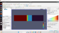
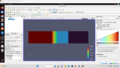
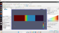
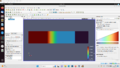
Now, we will investigate the influence of convection and diffusion terms on the temperature field of the fluid flow by changing the boundary conditions through modifying "T" and "U" files in the "0" folder of the "forwardStep". The following pictures (from left to right) represent the temperature field of the fluid flow under pure convection, pure diffusion, and the combination of convection and diffusion respectively.


To simulate the pure diffusion condition, the temperature has been considered equal to zero all over the domain except the left wall which is set to 10 Kelvin, the velocity is equal to zero all over the domain and the diffusivity has been set to 0.05. In contrast, to simulate pure convection, the velocity is equal to 0.2 m/s in the positive x direction with the inlet temperature of 10 Kelvin, and the diffusivity is equal to zero. Finally, to show the combination of diffusion and convection effects, the velocity is implemented equal to 0.2 m/s in the negative x direction, and the diffusivity is set to 0.05. It is interesting to note that some fundamental issues can be seen in the result of pure convection which is related to the discretization and the numerical methods applied in the simulation. In the following sections, we will talk about the differences between these schemes and their influence on the solution.