This page was developed by the Queen's University Applied Sustainability Research Group.

Operational Instructions for PhotoVoltaic and Trigeneration Optimisation  Model (PVTOM)

Introduction

PVTOM was developed to simulate and optimize hybrid photovoltaic and trigeneration energy systems based on technical, economic, and emissions performance. The theory and development of the model is documented in Nosrat, A.H. (2010) "Simulation and Optimization of Hybrid Photovoltaic (PV) and Combined Cooling, Heating, and Power Systems", Master's Thesis Dissertation submitted to Mechanical and Materials Engineering Department. Queen's University, Kingston, ON. Submitted on Dec. 24, 2010.

The following page are basic instructions on how to operate PVTOM.

The following page contains basic instructions on how to operate PVTOM. Currently, PVTOM requires MATLAB 2008 or later to operate. Additionally, you will require the optimization toolbox containing the multiga optimization tool. NOTE for reader: You CANNOT work with .xlsx files. Save all Excel spreadsheets in .xls format.

Step 1- Collect and Organize Input Data

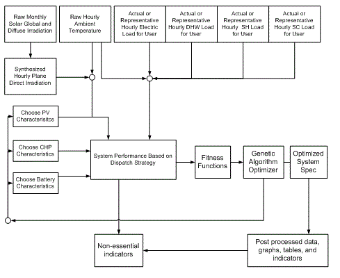
Explanation: According the flowchart presented as Figure 4.1 in the original thesis, PVTOM requires 6 inputs for every hour of the year to simulate and optimize a PV-Trigeneration. Additionally, it requires a set of characteristics for each of the three different technologies (PV, CHP, and batteries) subject to optimization. While PVTOM can upload this data for its use, it cannot provide the data beforehand. There are three primary sources for collecting input information: Generated hourly solar irradiation accessed by PVSyst 4.36, as high as 5-minute resolution data for temperature, space cooling, space heating, domestic hot water, and electric end-user requirements for a case study through the CHREM, and technology specifications through literature and commercial documents. There is no ‘clear’ set of instructions on obtaining this and would require some diligence from the developer to obtain pertinent information. There are instructions made available by PVSyst for exporting hourly irradiation data for different locations. The current structure for organizing data is certainly not set in stone and was developed to shifting priorities and information. Therefore, the user must ensure compatibility between organizing data and PVTOM’s uploading capabilities. It’s important to know that any ‘xlsread’ function in MATLAB is collecting data from an Excel (97-2003) file for a particular input parameter required for the operation of PVTOM. Therefore, understanding how the ‘xlsread’ function works and how it collects data is critical in preventing erroneous data collection. It is recommended that the input data be stored in Excel in the current format until such time the user is comfortable in altering the structure of the information.

Because there are a multitude of ways for collecting input data, it is near impossible to offer a step-by-step checklist on how to collect and organize input data.

NOTE: Currently, PVTOM cannot calculate tilted global irradiation for sloped surfaces from horizontal global irradiation. Therefore, the user must ensure global tilted irradiation for the optimum inclination angle of the given geographic region. Developers of PVTOM can include the capability of calculating tilted global irradiation from horizontal global irradiation based on Equation 19 of the original thesis.

 Step 2- Make sure all important files are in one folder

Explanation: All of PVTOM`s critical m-files and data files must be place in one folder. This folder is referred to as the directory folder. A quick way to view or change the current directory is by using the current directory field in the desktop toolbar. If you know or have copied the path for the new current directory, enter it in the field and press Enter. To look for a folder, click the Browse for Folder button.

Instructional Checklist: Ensure that your Current Directory is set to the same path as the directory folder. As of January 24, 2011, critical m-files that must be included in the directory folder include:

1. datauploadb.m (used for reading and archiving hourly temperature, solar irradiation, hourly end-user consumption data for SD and DR houses in 5 different Canadian cities.)
2. technologies.m (for uploading technology specifications for PV, CHP, and battery technologies)
3. optimmasterversion.m (This m-file is the ‘interaction point’ between MATLAB’s ‘multiga’ multiobjective genetic algorithm function and the dispatch strategy based on technologies, solar irradiation, temperature, and end0user requirements.)
4. costs.m (this m-file is called upon in optimmasterversion to do life cycle cost calculations).

indicators.m (used for post-optimization analysis of various systems)
As of January 24, 2011, critical Excel (97-2003) files include:

1. ‘five datasets’ (30-minute resolution data of end-user requirements for the 10 different case studies used in thesis)
2. ‘pvsyst_radiation_and_temp’ (hourly irradiation and temperature obtained from PVSyst)
3. ‘technologies’ (characteristics of PV, CHP, and Battery technologies)
   

Step 3- Load Technologies

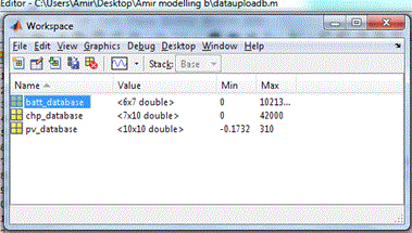
 Explanation: You can tabulate your technology specifications in technologies.xls. The PV, CHP, and batteries are in separate sheets. For example, if you wish to enter a PV technology by the theoretical name of ‘ACME PV100’, you would enter the technology parameters in row 21 in spreadsheet ‘PV’. For PVTOM, columns H, O to T, AN, and BA must be completed. You can add a CHP technology in its respective spreadsheet by tabulating parameters in column J and beyond. The CHP spreadsheet must have rows 9-12, 14-18 filled out. If you want to add a battery, you can expand the database starting from row 12. Finally, you need to ensure that the reading ranges of the MATLAB function ‘xlsread’ in lines 11-14 of ‘technologies.m’ correspond to the array size of the corresponding spreadsheets. For example, if the PV database starts at row 11 and ends at row 21, all range values for ‘xlsread’ defined in pv_database must be set to ‘Column11:Column21’ instead of the current ‘Column11:Column20’. The ‘technologies’ m-file automatically uploads and saves the technology parameters in three MATLAB data arrays named as pv_database, chp_database, and batt_database. Theoretically speaking, the m-file assigns a number for each technology (by its location in the particular column or row). Once optimized, the ‘assigned number’ must then be corresponded with the original Excel spreadsheet to determine the specific technology. For example, assigned number 1 for the battery calls Hoppecke 10 OPzS 1000 and all of its specifications. Assigned number 6 calls Vision 6FM55D, and so on.

Instructional Checklist:

1. Open MATLAB.
2. Open the ‘technologies’ m-file by typing ‘open technologies’ in the MATLAB Command Window.
3.  Press the Run button (It looks like a green arrow    ) or F5 . After a few seconds, you should see three data arrays in the MATLAB Workspace Toolbar named as ‘pv_database’, ‘chp_database’, ‘batt_database’.
   
   

Step 4- Load Solar Irradiation, Temperature, and End-User Requirements

Explanation: PVTOM includes an m-file that uploads and organizes the solar irradiation, temperature, and end-user requirements of different As it stands now, the `datauploadb` m-file uploads data identically for the 10 different case studies used in the thesis. For each case study, the m-file retrieves data from the particular excel spreadsheet containing information about the particular case study. There is a unique method for collecting data that is repeated for each case study. The m-file code distinguishes which case study it`s working on based on the green text (ie. %Kingston DR). First, it asks for the grid emission intensity (used based on province) located in cell J3 of every spreadsheet in pvsyst_radiation_and_temp.xls. Then it uploads CHREM`s thirty-minute resolution end-user data from `five datasets.xls` in cells E2:M17521. Next, it uploads global solar irradiation on a tilted plane from cells G9:G8768 of pvsyst_radiation_and_temp.xls (note: the model does not yet convert global to tilted even though the formula was written in the thesis; as such tilted global irradiation outputs were obtained directly from PVSyst for an angle of 30 degrees at each of the five locations). Finally, it will upload hourly ambient temperature from H9:H8768 of pvsyst_radiation_and_temp.xls.
The m-file then compresses the 30-minute end-user data into hourly data. It then saves all of these inputs in the following format: `cityname`data`housetype`. For example, data for a DR house in Kingston will be archived as kingstondatadr. It is recommended that new case studies follow the same data processing and archiving structure. You can remove a case study by deleting the block associated with the particular location. You can add a case study by copying and modifying the same structure to a particular case study. You must collect and organize the information in the pertinent Excel files beforehand.

NOTE A: There seems to be a discrepancy between different versions of MATLAB between the ‘rem’ and ‘frac’ functions. Some can read the former and some the latter. The reader is encouraged to understand their functionality independent of these instructions. In practical terms, the compression of the 30-minute resolution into hourly resolution requires either function. If you see an error indicating that MATLAB doesn’t recognize ‘rem’ (ie. MATLAB command window says “??? Undefined function or variable ‘rem'”), line 16 of ‘datauploadb.m’ (as well as all corresponding lines for each case study data upload) should read:
if frac(sym(n/2))==0
Otherwise, if MATLAB doesn’t recognize ‘frac’, line 16 should read:
if rem(n,2)==0

You can use the find & replace function in MATLAB (cntrl+F) to do this for a large number of case studies.

NOTE B: The CHREM is capable of producing as high as 5-minute resolution data. The thesis used 30-minute resolution data. The reader can effectively compress any resolution to a lower resolution within lines 14-22 (and corresponding lines for each case study). As the possibilities are innumerable, the reader is encouraged to modify these with their knowledge of MATLAB and independent of this set of instructions.
Instructional Checklist:

1. Open ‘datauploadb.m’.
2. Ensure line 16 and all corresponding lines are supported by your version of MATLAB (See NOTE A)
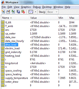
3. Press the Run button or F5. If the m-file runs properly, you should now be able to load the six inputs required for each geographical location. You can test the veracity of your uploaded data by typing ‘load’ followed by the case study data archive name in the MATLAB command window. For the SD house in Kingston, you can type ‘load kingstondatasd’. You should see 18 data arrays in your workspace (see below; some are non-essential to PVTOM). You can read the data in each data array by double-clicking on the respective icon. You should have the same arrays for every case study.The data upload process is complete when you see a plot function representing the hourly end-use energy consumption for the last case study. The blue line represents electricity, red represents space heating, green represents domestic hot water, and light blue represents space heating.